Alternative Retirement Investments for Farmers
August 18, 1996
PAER-1996-4
George F. Patrick, Extension Economist and Christine M. Hamaker, former Research Assistant
![]()
![]()
![]()
![]()
![]()
Many farmers do little formal planning or investing specifically for retirement. Typically, any sur-plus funds are reinvested in the farm operation with the hope that the farm will provide the necessary retirement income. However, the experiences of the 1980’s indicate that wealth held as farm assets is very vulnerable to changes in the agricultural economy. Total equity in farm real estate dropped nearly 40 percent from $686 billion in December 1981 to $422 billion in 1986. Thus, a more diversified investment portfolio may provide a more secure retirement.
Retirement planning for farmers is important for a number of rea-sons. In farm operations involving more than one generation, farm assets may be inadequate to provide sufficient income for both generations as the retiring farmer’s labor input is reduced. The question of
“How big a retirement income the farm will provide” is generally an issue. Other farm families may be concerned about outliving the accumulated assets in their retirement portfolio.
This study analyses the effects of alternative retirement investment strategies based on their performance during the 1965 to 1991 period. Although future performance is unknown, the past may be the best indicator available. The study examines the value of the portfolio accumulated for retirement, the level of retirement income generated, and the probabilities of using up or exhausting the accumulated portfolio during a 20-year retirement period. The study is not intended to develop an optimal retirement strategy for farmers or retirement investment strategies for individual farm families. However, the results obtained may be useful guidelines for farm families in their retirement planning.
Overview of the Simulation Model A spreadsheet is used to simulate farm financial performance over a 20-year period of pre-retirement accumulation and a 20-year retirement period in real terms (adjusted for inflation). Based on the initial conditions specified, the model deter-mines farm income, reinvestment necessary to maintain the farm operation, funds available for additional investment, and other variables each year. If funds are available for additional investment, they are allocated as specified in the investment strategies being analyzed. At retirement, current and non-land farm assets are liquidated over three years to reduce taxes, and the farm real estate is cash rented. Social security benefits equal to the average benefits received by a couple in 1993 are included as retirement income. In addition, if there are any other investments, the returns from these investments are also included in their retirement income, and taxes are calculated. If the total after-tax retirement income exceeds necessary loan payments and family living expenses, the excess reduces existing loans or is invested in a money market account. If the total after-tax retirement income does not meet loan repayments and family living expenses, the deficit is drawn from the money market account or by borrowing against other farm and nonfarm assets.
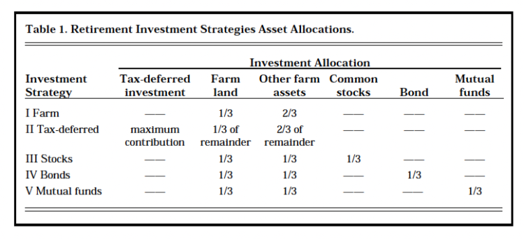
Table 1. Retirement Investment Strategies Asset Allocations.
All of the analysis is in real terms, in 1993 dollars. Thus, a dollar received at the end of the 20-year retirement period has the same purchasing power as dollar at the beginning of the 20-year pre-retirement period. The distributions of the current and capital gains portions of the returns used in the model are based on the average returns and the variability of returns experienced during the 1965 to 1991 period. For each year in the simulation, the returns to the various investments are randomly drawn from these distributions. Thus, there could be a series of good or bad years. A total of 500 replications of each strategy are used to obtain information about the range of possible outcomes.
Alternative Retirement Investment Strategies
Five alternative investment strategies (Table 1) are analyzed. All of the retirement investment strategies involve some additional investment in the farm operation if funds in excess of capital replacement needs of the current farm are available. In Strategy I, all available funds are reinvested in the farm operation. One-third is invested in land and the remaining amount is divided, 40 percent for current assets and 60 percent for intermediate assets (listed as Other farm assets). In Strategy II, if available funds permit, the maximum allowable contribution is made into a tax-deferred individual retirement account, IRA or Keogh plan. Any remaining funds are invested as in Strategy I. The last three strategies allocate two-thirds of available funds into farmland and other farm assets as in Strategy I and one-third into common stocks, U.S. bonds, or growth stock mutual funds, respectively.
The averages and variability of the annual current, capital gain, and total returns of the alternative investments for the 1965 to 1991 period are in Table 2. Current returns are the net operating returns from farming, the dividends from stock, and the interest from bonds. Capital gain returns are the changes in the values of the assets, while the total return is the sum of the current and capital gain returns of an investment. Average real current returns varied from 2.25 percent for growth mutual funds to 7.70 percent for U.S. bonds. Average real capital gain returns of whole farm and U.S. bond investments were negative, while growth stocks returned 4.01 percent annually.
Variability is indicated by the standard deviation. If the distribution of returns, say for U.S. bonds, follows the bell-shaped normal curve, then real current returns from bonds would be expected to be in the range of 5.59 to 9.81 percent (7.70%, + or -2.11%) more than two-thirds of the years. The capital gains portion of the returns is much more variable than the current returns portion for all of the investments considered. The current, capital gain, and total returns of agricultural investments were negatively correlated with stocks, bonds, and mutual funds. Thus, an investment split between agricultural and non-farm investments will have a more stable return than a non-diversified investment.
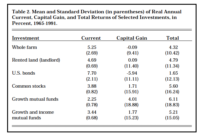
Table 2. Mean and Standard Deviation (in parentheses) of Real Annual Current, Capital Gain, and Total Returns of Selected Investments, in Percent, 1965-1991.
Base Situation
For this study, a couple, each 45 years old, with assets similar to the average of participants in 1992 Indiana comparative farm business summary is assumed. They plan to retire at age 65, are not interested in transferring the farm to other family members, and want to maintain an after-tax level of real family living expenditures of about $27,800 per year. Three initial situations, representing different wealth positions, are analyzed. The net worth positions represent three levels of owned acreage: 240, 320, and 400 acres. All farms had debt/asset ratios of 45 per-cent and $244,845 in intermediate debt. The amount of long-term debt varies with the owned acreage. The net worths are $461,650, $542,610, and $736,000, respectively.
In the base simulation, it is assumed averaged real returns in pre- and post-retirement periods would be the same as real returns had been for the 1965 to 1991 period with the same variability. As noted previously, the real capital gain to land was negative, -0.09 percent annually, during the period. An alternative scenario, with the real capital gain in land values increasing 0.09 percent annually and greater variability of current returns to the whole farm investment, was also simulated.
Simulation Results
Because results are generally simi-lar, only the middle situation -the 320 owned acres and initial net worth of $543,000 – is presented in Table 3. In the base simulation, on average, all of the investment strategies had growth in real terms over the 20 year period. The largest average portfolio at the beginning of retirement resulted from Strategy II, the tax-deferred investment. The beginning retirement portfolio was almost $100,000 larger than the second place strategy, mutual fund investment (Strategy V), and nearly 20 percent larger than strictly rein-vesting in the farm operation (Strategy I). The tax-deferred investment strategy also resulted in both the highest maximum (best) and mini-mum (worst) ending portfolios. Growth mutual funds performed better than stocks, while bonds (Strategy IV) were the poorest performing investment. The negative minimum value indicates the family would have “gone broke” before retiring in the worst case.
In the alternative scenario simulation, when the variability of cur-rent returns to farm operation and real capital gains to farmland are increased, differences among the beginning retirement portfolios from the alternative investment strategies are reduced. This is because farmland is the major asset in all of the portfolios, and land increases in real value over time.
The tax-deferred investment strategy continues to provide the largest aver-age portfolio and the largest standard deviation. The farm investment strategy remains at fourth but now is only about 13 percent behind tax-deferred investments. Investment in bonds continues to be the poorest performing portfolio.
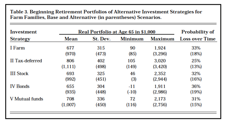
Table 3. Beginning Retirement Portfolios of Alternative Investment Strategies for Farm Families, Base and Alternative (in parentheses) Scenarios.
The right hand column of Table 3 indicates the probability that the beginning retirement portfolio value, or wealth at age 65, would be less than it was initially at age 45. In the base simulation, the probabilities ranged from 25 percent for Strategy II, tax deferred investments, to 36 percent for Strategy IV, the bond investment strategy. These results imply that if the variability of future investment performance is the same as it was over the 1965-1991 period, all investment strategies have a substantial probability, 25 to 36 percent chance, of losing value in real terms before the farm couple reaches age 65. For the sensitivity analysis, with increased variability of current farm returns and increased real land values, the probabilities of “losing ground” are lower. However, the probabilities still range from 13 to 19 percent.
Value After 20 Years of Retirement The portfolio performance and ending portfolio value after 20 years of retirement are also simulated 500 times to generate information on the range of possible outcomes. For the tax-deferred strategy, Strategy II, it is assumed that a capital distribution is made each year beginning at age 65. The distribution is calculated by dividing the value of the IRA/Keogh plan at the beginning of the year by the remaining joint life expectancy of the couple. In retirement, it is assumed that all families receive $11,700 in social security benefits annually. If social security and income from rent and investments does not provide $27,800 for family living after taxes and necessary loan repayment, then the couple will borrow against their investment portfolio of farm and nonfarm assets.
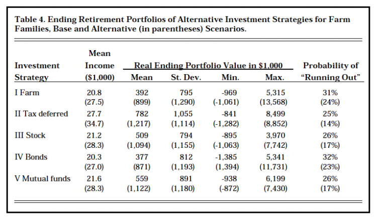
Table 4. Ending Retirement Portfolios of Alternative Investment Strategies for Farm Families, Base and Alternative (in parentheses) Scenarios.
The average retirement incomes and ending portfolios for the different retirement investment strategies in the base and alternative scenario simulations are presented in Table 4. None of the investment strategies in the base simulation, on average, provide the specified level of family living. Strategy II, the tax deferred IRA/Koegh investment, comes closest, in part because of the capital distribution. However, on average, the tax-deferred investment strategy has the smallest decrease in value over the retirement period. All of the other investment strategies provide aver-age incomes of $20,300 to $21,600 and require the couple to borrow against the assets in their retirement portfolio.
Strategy I, reinvestment in the farm operation, and Strategy IV, investment in bonds, have the largest average reductions in portfolio value during retirement. These investment strategies are the least able to provide for retirement income without invading the principal. Because of the higher real land values in the alternative scenario, all of the retirement investment strategies provide average retirement incomes which are very close to or exceed the $27,800 level of fam-ily living. The tax-deferred investment strategy provides the highest level of income, again in part, because of the required capital distribution. However, a comparison of Tables 3 and 4 indicates that the tax-deferred investment strategy portfolio increases in average real value over the 20-year retirement period.
The risk of exhausting the retirement portfolio or “running out” of retirement funds, without changes in family living expenditures, before the end of the 20-year retirement period ranges from 25 to 32 percent in the base simulation. All of the retirement investment strategies involve a majority of farm investments which decline slightly in real value over time. In the alternative scenario, when real land values increase slightly, the prob-abilities of exhausting the retirement portfolio before the end of 20-year retirement period are reduced. However, even in this case, there is a 14 to 24 percent chance of the retirement portfolio being exhausted.
Conclusions and Implications Results of this study indicate that diversified retirement investment strategies, especially tax-deferred investments, generally result in larger retirement portfolios and higher retirement incomes than rein-vestment of all available funds into the farm operation. In the base simulation, which involved a slight decrease in real land values, none of the investment strategies provide the specified level of family living, on average, without some borrowing against assets for the farms starting with 240 and 320 owned acres. Only the tax-deferred retirement strategy provided the specified level of family living for the farm starting with 400 acres. The reinvestment in farm assets strategy led to average beginning retirement portfolios of $674,000, $806,000, and $932,000, before contingent tax liabilities, for the farms starting with 240, 320, and 400 owned acres, respectively. These retirement portfolios, which are equivalent to net worth, are substantial by most standards yet do not allow the retired couple “to live off of the income from the farm.”
There is a substantial chance, 25 to 40 percent in the base simulation, that the real value of the investment portfolio will decline during the 20-year pre-retirement accumulation period. In some instances the value of the portfolio at the beginning of retirement is negative, suggesting that the couple is bankrupt. However, the model does not allow withdrawal from farming, part or full-time nonfarm employment by one or both spouses, or other responses which farm families might make when faced with deteriorating economic conditions.
The probabilities of exhausting the retirement portfolio over the 20-year retirement period range from 25 to 32 percent in the base simulation. The variability associated with the current returns and capital gains in the agricultural sec-tor over the 1965 to 1991 period was very large. Both the run-up in land values and high farm incomes of the 1970’s as well as the drastic decline in land values and negative incomes of the 1980s are included. A more stable period would result in less extreme values, on both the high as well as the low side. However, even with more optimistic assumptions about farm land values, the prob-ability of “running out” or exhausting the retirement portfolio over a 20 year period is always 12 percent or higher.
This study emphasizes the need for retirement investment planning, especially with respect to the beneficial effects of tax=deferred retirement investments. Furthermore, the results also suggest the need for farm families to plan their retirement income and expenses. Many farm families will need to consider significant changes in family living expenditures, delayed retirement, or other responses in retirement to avoid exhausting their retirement portfolio.
![]()
![]()
![]()
![]()
![]()