Are Current Farmland Values Reasonable?
June 23, 2011
PAER-2011-01
Craig Dobbins, Brent Gloy, Michael Boehlje, and Chris Hurt, Professors
![]()
![]()
![]()
![]()
![]()
Introduction
In recent months, there have been several reports of strong increases in farmland values. Fourth quarter Federal Reserve Bank of Kansas City survey results indicate an annual increase of 17.6% and 17.5% for irrigated and non-irrigated farmland in Nebraska. The annual increase for non-irrigated farmland in Kansas was even stronger at 19.5%1. In Iowa, Indiana, and Illinois, the Chicago Federal Reserve Bank survey reported annual increases of 18%, 12%, and 11%, respectively2. These increases follow a long-term trend of rising farmland values – since 1985 Indiana land values have increased by 270%, a compounded growth rate of 5.4% per year. These large increases have created considerable debate about the level of current farmland prices and what the future might hold.
There are several drivers that influence farmland values. One key factor of the farmland market is the net return from crop production, currently at historical highs. However, farmland markets are also influenced by factors such as the potential conversion of farmland to urban development, qualification as like-kind property in federal tax law Section1031 tax-deferred exchanges, and capital gain tax policy. It is also important to recognize that annual farmland transactions are a small amount of the total farmland available, making this a market where the value of only a few transactions is generalized to the whole. Financial forces such as interest rates and alternative investments also exert an influence on farmland values. Expectations about these financial forces and future earnings strongly influence market activity and farmland price.
While all these factors are important, this discussion focuses on the returns and financial forces influencing farmland values. This discussion also suggests a structure that helps organize thinking about how returns and financial forces interact and impact farmland values.
Structuring Farmland Value Thinking with Income Capitalization
Farmland is a capital asset, and people generally buy capital assets to obtain the future earnings associated with asset use. Since money is being spent today for future income, the future income needs to be adjusted to a current value. Because we must wait for the income from our purchase of farmland, future income is worth less to us than income received today. This occurs for several reasons. First there is inflation; future income will buy fewer goods than income today. There is also the time value of money. If we had the income today, we could invest it and have more income in the future. Or we could choose to spend the income and obtain the benefits of the goods purchased today. Finally, there is risk, the risk that the future income is not as much as expected, or worse, there is no future income.
Because the evaluation of a capital investment is so common, analytical models have been developed. One of these models is income capitalization for a capital asset with an infinite life (Equation 1, below). Assuming the asset has an infinite life simplifies the model. If farmland is properly maintained, farmland may be an infinite life asset. Farmland will generate income for the current owner and for future owners. This assumption also means that the income level for owning farmland and the growth rate in farmland income must be realistic for a very long run. In periods of relatively high crop prices expectations about income levels and changes in income may become overly optimistic.

Equation 1. Farmland Value
This income capitalization model says that farmland value is determined by the income generated from owning the asset, the interest rate on low-risk securities such as 10-year Treasury bonds, a risk premium, and the growth rate of income. The interest rate plus the risk premium represents the discount rate, the rate used to adjust expected future income. In this model, increases in farmland values can come from increases in income, decreases in the discount rate, or increases in the growth rate of farmland income. Each of these factors is discussed.
Income
Income in Equation 1 represents the net return to a farmland owner. This is the net income remaining from crop production after all expenses except the return on the farmland investment have been subtracted from revenues. This means crop production inputs, investments in machinery and equipment, operator and family labor, and farmland maintenance costs are included as expenses. The capitalization model indicates a positive relationship between income and farmland value–the greater farmland income, the greater the farmland value.
A major contributor to current farmland income is high crop prices. Beware, increases in crop prices are often followed by increases in fertilizer, seed, chemical, and other input prices. Crop price increases a few years ago were accompanied by fertilizer prices in excess of $1,000 per ton and significant increases in seed and other crop input prices. As a result, when thinking about income from farmland ownership, it is important to focus on the net that remains from crop production after all resources except farmland have received a payment. In many cases, cash rent is used as a proxy for this return.
Discount rate
The discount rate can be thought of as the rate of interest on low-risk securities plus an upward adjustment for farmland investment risk. The discount rate represents the opportunity cost of owning a risky asset. Factors such as expected future inflation, borrowing costs, and rates of return on alternative investments affect the opportunity cost. A relevant opportunity cost is the interest rate on farm loans. By using cash to pay down debt rather than buy farmland, the farmer is assured of a “return” equal to the debt interest rate. The rate that could be earned on an investment of comparable risk is another way to think of the opportunity cost.
The discount rate recognizes and implements the time value of money–future income is not worth as much today as current income. This is an important concept because the income from a farmland investment will be received over a number of years. The discount rate adjusts expected future income to a current value.
Interest rates on 10-year Treasury bonds are often used to represent the interest rate of low-risk securities.
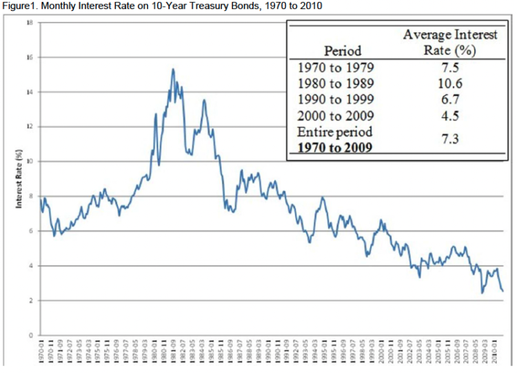
Figure 1. Monthly Interest Rate on 10-Year Treasury Bonds, 1970 to 2010
Figure 1 shows the average interest rate on 10-year U.S. Treasury bonds issued over the period of 1970 to 2010. Rates fluctuated widely over this period. Starting at roughly 8%, in 1970, rates started to climb, reaching a peak of 15% in the early 1980’s. Since peaking, they have declined to slightly less than 3% today. While the exact impact of interest rates on farmland prices is difficult to measure, the high interest rates of the early 1980s are associated with large declines in farmland values between 1981 and 1986. Since 1986, declining interest rates have been associated with steadily rising farmland values. Other things equal, higher long-term interest rates and risk premiums will decrease farmland values.
Growth rate
The growth rate used in the capitalization model is the rate at which farmland income is expected to grow. Factors that influence the growth rate are productivity gains associated with higher yields and inflation. The difference between the discount rate and the growth rate is often referred to as the capitalization rate or “cap rate.” The capitalization model shows that there is a positive relationship with the value of farmland and the income growth rate. An expected higher growth rate from farmland income brings a willingness to pay more for farmland, other things being the same. If the expected growth rate in income declines, farmland becomes less valuable.
Cash rents are often used as a proxy for the net income from farmland. The Purdue Land Value Survey indicates that for the period of 1975 to 2010, cash rent on average land increased at an annual, compound rate of 2.7%. Starting in 1987 produces an annual compound growth rate of 3.6%. For 2000-2010, cash rents grew 3.7% annually, and from 2005-2010 the growth rate was 5.0%.
The Relationship Between Farmland Value and Earnings
While a number of different ways of describing the relationship between farmland income and farmland prices have been developed, the value to income multiple or price to earnings (P/E) ratio is one of the most common. The P/E ratio describes how much buyers are willing to pay for each dollar of income. As a matter of convenience, earnings (E) are usually estimated as either the most recent level of income, the income forecast for the upcoming year, or the current or expected future cash rent.
The income capitalization model is directly related to the farmland price to earnings ratio (income multiple). The price to earnings ratio can be found by dividing Equation 1 by income:
Thus, the income multiple is the inverse of the capitalization rate.

Equation 2: Farmland Value over Income
If the risk premium and income growth rate remain constant, a decline in the long-term interest rate decreases the capitalization rate and increases the associated earnings multiple and farmland value. One must also consider how the risk premium that investors associate with farmland has changed as well. Lower capitalization rates, and higher multiples, could also be achieved by investors requiring a smaller risk premium or by expecting a higher rate of growth in farm income.
The relationship between the 10-year Treasury rate, the growth rate, and risk premium is illustrated in Table 1. The cash rent multiple for average quality Indiana farmland is shown for selected years. The average annual interest rate on the 10-year U.S. Treasury is used as a proxy for the long-term return and is shown in the next column.
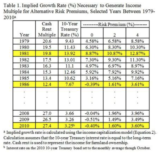
Table 1. Implied Growth Rate (%) Necessary to Generate Income Multiple for Alternative Risk Premiums, Selected Years Between 1979-2010
The subsequent columns show the implied growth rate in income necessary to generate the income multiple under alternative assumptions about the risk premium.
For example, in 1981 the cash rent multiple was 19.8. Given the 10-year Treasury rate of 13.92%, if investors require a risk premium of 2%, the implied annual growth rate in income is 10.87%. While inflation rates were high at that time, a long-lasting growth rate of over 10% for farmland income turned out to be much too optimistic. By the time the downward adjustment in farmland values was complete in 1987, the needed annual increase in farmland income with a 2% risk premium had declined to 1.61%.
Figure 2 graphically illustrates the implied income growth rates under no risk premium, 2% risk premium, and 4% risk premium scenarios. Here, one can clearly see the very large implied income growth rates of the late 1970’s and early 1980’s. Valuing farmland using the income capitalization model suggests that investor expectations for future income growth were overly optimistic.
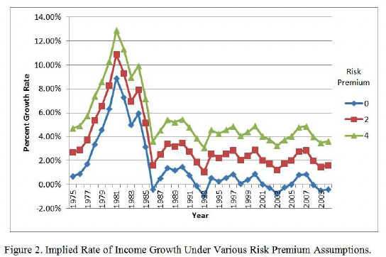
Figure 2. Implied Rate of Income Growth Under Various Risk Premium Assumptions
In 2010, the current combination of interest rates on 10-year Treasury bonds, a 2% risk premium, and farmland values for average land in Indiana results in an implied growth rate of 1.6%, nearly the same as 1986. However, with the increased variability in income, it is expected that the risk premium for many investors, especially the owner-operator investor, has increased. If there is a risk premium of 4% in the market, a growth rate of 3.6% is required to justify the current farmland value/income relationship.
Final Comments
At the March meeting of the Indiana Society of Farm Managers and Rural Appraisers, attendees were asked to estimate the current value of 80 acres with long-term corn and soybean yields of 165 and 50 bushels per acre, respectively. The average value for such a tract was $6,028 per acre. The attendees were also asked to estimate the current cash rent. The average cash rent was $208 per acre. This would provide a current income multiple of 30.
Given a10-year Treasury rate of 3.25%, a cash rent multiple of this size implies an income growth rate of 1.93%. Will these expectations about continued low interest rates, strong income, and moderate income growth rates be realized?
Expected farmland earnings, interest rates, risk premiums, and farmland income growth rates have all been favorable in recent times. Crop income has been larger than historical averages and growing faster than historical rates due to increased demand for bio-fuels, export demand growth from developing countries, and a weaker dollar. While it is difficult to forecast the effect of these variables on crop prices in the future, it appears that at least in the area of biofuels, the massive demand expansion is likely to moderate. Current farmland income is also likely to decline because of increases in crop production costs.
![]()
![]()
![]()
![]()
![]()