Clues to Future Crop Economics From the Past
April 12, 2015
PAER-2015-3
Chris Hurt, Professor of Agricultural Economics
![]()
![]()
![]()
![]()
![]()
U.S. and global crop agriculture seems to be in a downward transition from record high economic activity during 2010 to 2013. Not surprisingly, the current downward adjustments are likely just a portion of a longer run cycle.
This longer term cycle is most closely correlated with the prices of commodities. Prices of course are determined by both supply and demand forces. Prices are also strongly related to the amount of economic activity in an industry with the initial upward price movement in commodity prices resulting in high returns to producers which in turn encourage them to increase demand for crop resources like machinery, fertilizer and land. Over time, however, the higher commodity prices result in a production response and increasing production. High commodity prices also have demand impacts providing incentives to reduce consumption quantities.
Figure 1 is an illustration of a hypothetical 29 year commodity cycle. Index numbers are used to provide a rough illustration of the magnitudes of economic activity. Starting from the left hand side, the index of economic activity is 100.
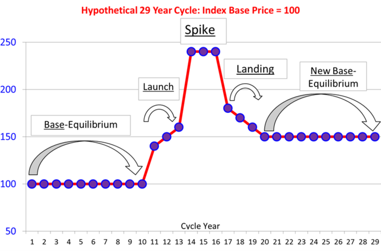
Figure 1. Hypothetical Price Cycle
The 29 year cycle is divided into five periods. The first is about 10 years of relative stability in a base equilibrium. The launch represents a few years were some new demand forces begin to drive prices and economic activity higher. The third period is the spike where the peak of the cycle occurs and economic activity may reach double or even triple the levels of the base. A common phrase heard in the industry is “we are now in a new era.” The landing is a period when supply is catching up to demand surges, and prices are moderating. Finally the new long-run equilibrium may be a fairly long period as represented by roughly 10 years in the illustration. Generally the new base equilibrium is at a higher level than the original equilibrium and is illustrated as about 1.5 time the base period.
This long term 29 year cycle has about 1/3 of the time in the base equilibrium, about 1/3 of the time in the sharp rise and then moderation, and about 1/3 of the time in the new equilibrium. It is important to recognize that the exact pattern of any cycle is dependent upon the specific conditions that affect supply and demand during that cycle. This means that the lengths may be different across cycles and the magnitude of increase and decrease can vary in different cycles. This also means that using past cycle behavior to forecast the current and future patterns should be used with great caution. This is because the economic conditions that will prevail in upcoming years cannot be known with certainty, but will evolve as time progresses.
Finally, we will look at past cycle behavior to try to gain some clues about the future of crop economics. Most in agriculture are aware that past cycles have exhibited “boom and bust” tendencies for economic activity. However, we will soon find that is not always the case, and another possible pattern observed in history is a “boom and moderation” cycle. How will the current cycle end? The answer will be determined over coming years and will depend on a host of factors we will discuss.
Historical U.S. Corn Cycle
To gain some insight into the historical economic crop cycles, we will use corn revenue per acre adjusted for inflation (real revenues). Adjusting for inflation is necessary when looking at revenues over more than 100 years because of substantial changes in the buying power of the currency. Corn revenue per acre is used as a proxy for the economic activity generated from an average acre of national corn production. USDA maintains yield per acre and U.S. corn prices received by farmers back many years. This analysis begins in 1900 and projects revenues per acre through 2018 based on average trend yields for the 2015 to 2018 crops and uses current corn futures prices to estimate average cash prices received for the 2015 to 2018 crops. All revenues per acre are then deflated using the Consumer Price Index and 2015 prices (current prices). Government program payments are not included in these revenues, but crop insurance proceeds are included.
Figure 1 shows these real U.S. revenues per acre for 1900 to 2018. The first observation is the enormous range from $131 per acre in the Great Depression year of 1931 to $1,248 per acre in 1973 during the 70’s boom. Keep in mind that the $131 per acre is in current 2015 dollars.
You can also note the upward moving trend line through the real revenues. Agriculture production technology has changed drastically over this period and one interpretation of the trend line is that this technology has enabled each acre of corn to produce more economic output in real (inflation adjusted) terms. So comparing 1931 to 1973 needs to be done in relationship to the trend.
A second interpretation of the trend line is that it represents some aspects of an average costs of production over this very long period. Data on costs of production is simply not available over this long period. If one uses the trend line as a rough proxy for costs over time, it may shed some light in evaluating returns during various periods of time. Again this is a rough proxy, but when revenues are well above the trend line odds are high that this was a very favorable return period for U.S. corn farmers. And when revenues are well below the trend line, this likely indicates a period when returns were low and perhaps negative.
There are four long term cycles. The first cycle is the period represented by World War I and the agricultural depression years of the 1920 and 1930s. The peak year was 1917 when real revenues reached $678 per acre in current dollars, and busted to just $172 by 1921. We see clear characteristics of the hypothetical 29 year cycle. Real revenues in the early 1900s were about $300 to $400 per acre. Then the new food export demands to feed war-torn Europe pushed real revenues per acre up $600 to $700. U.S. farmers responded by “plowing up the plains,” bringing millions of new acres into production. When the war was over, exports to Europe fell greatly reducing demand for U.S. crops. European farmers went back to production, but the new acreage in the U.S. did not drop out of production. This created an imbalance of excess supply in relationship to demand with farm level prices below costs of production. Other characteristics of the period were plummeting farm incomes, falling land values, and economic recession/depression in U.S. agriculture.
The second cycle boom was around World War II and included the 1950’s and 1960’s after. The figure clearly shows how World War II finally helped raise economic activity out of the great depression lows. Real corn revenues in the 1930’s of $200 to $300 per acre lurched higher to $500 to $700 in the early and mid-1940’s. The downward adjustment in the 1950’s and 1960’s was not nearly as severe as after WW I.
While the WW I cycle was an extreme boom and bust cycle, the 1940’s to 1960’s cycle was more of a boom and moderation pattern, Why? Two potential explanations are that wage and price controls during WW II were fairly effective at preventing farm prices from rising as sharply as they might have in their absence. It stands to reason that if prices did not go so high in the boom, they did have to fall so much in the downward phase of the cycle. A second supporting argument is that world economic growth was strong after WW II as the world was rebuilding and recovering from the pent up demand that could not be satisfied in the great depression of the 1930’s. Strong world income growth in the 1950’s and 1960’s provided a stronger export base for U.S. crops and helped reduce the downside adjustments compared to the disaster after WW I. The important message from this cycle is that U.S. agriculture can have boom and moderation cycles. They do not have to end in busts.
The third cycle is the 1970’s and 1980’s boom and bust. Real corn revenues in the 1960’s were in the $500 to $700 range and boomed to about $1,100 an acre on average for the years 1973, 1974, and 1975. Corn and other commodity prices were caught up with massive macroeconomic factors that caused them to move sharply higher. The U.S. abandoned gold as the foundation of the dollar, sharply devaluating the buying power of the dollar. OPEC organized as a cartel to push up world oil prices and the former Soviet Union began to buy massive quantities of wheat and other basic food commodities in the world market. Inflationary monetary and fiscal policies of the U.S. also set off further inflationary pressures. Inflation of the 1970s sent crop prices higher, but gaining control of inflation in the 1980’s resulted in massive declines of crop prices and economic activity.
The real revenues that had been up to, and above, $1,000 per acre retreated to generally $400 to $500 from the mid-1980’s until 2005. Thus in the “new equilibrium” real revenues retreated to somewhat below where they were in the “base equilibrium” before the early 1970’s boom.
Both the WW I cycle and the 1970’s/1980’s cycle were boom and bust cycles. But the WW II cycle was much more of a boom and then moderation cycle. Thus our 100+ year history lesson shows two boom and bust cycles and one cycle of boom and moderation.
Characteristics of the Current Cycle
We have seen that cycle patterns and lengths are dependent on the forces at play during each individual cycle. What about the current cycle? A glance at Figure 2 shows that the base equilibrium period from 1998 to 2005 was the lowest period of real corn revenues dating back to the 1920’s and 1930’s. Crop margins were tight and there was little incentive for the world to invest in low-return crop production, yet world total usage was growing. This was thus a period when world ending inventories were dropping, but still considered adequate and therefore crop prices remained depressed.

Figure 2. U.S. Real Revenue Per Acre
At least three drivers began to change the global picture in the mid-2000’s. Global biofuels policies were to dramatically increase demand for feed stocks like corn and vegetable oils. In fact, one of the objectives of U.S. biofuels policy was to enhance economic activity in rural communities. The second factor was the enormous increase in soybean demand from China. Ag economists often broadly characterize this driver as “higher incomes in developing countries.” The third driver was macroeconomic policies that caused the U.S. dollar to be at 20 year lows at times during the 2008 to 2011 period. And finally, low yields in parts of the world during this period and low U.S. yields in 2010, 2011 and 2012 contributed to tight world inventories. Demand growth had exceed supply and as a result prices rose to ration a short supply situation.
As a result of inventory shortages and higher prices, real corn revenues per acre rose from $372 per acre in 2005 to a peak of $1,019 per acre in 2012 (with crop insurance indemnities included in revenues). The boom was in place. A return to better yields in the 2013/14 and 2014/15 crop years and a leveling-off of demand growth for biofuels has enabled the world to begin to restore inventories to more adequate levels with prices in moderation.
How Does the Current Cycle End?
We have seen that booms in economic activity in crop agriculture have occurred four times in the past 115 years. Real corn revenues per acre in 2015 dollars were used to illustrate these cycles that may be 30 years or longer. They are composed of a base equilibrium period, a period of surge, and then a period of downward adjustment as prices return to a more stable new equilibrium.
While history provides some general patterns and time lengths, each cycle’s parameters are determined by the unique events occurring at that time. The current cycle has clearly exhibited a boom phase when real corn revenues in the U.S. have more than doubled from the 1998 to 2005 base. Real corn revenues averaged $926 per acre during the four year period covering the 2010 to 2013 U.S. crops. The crops in 2013, 2014, and 2015 appear to be making a transition toward a much lower revenue average. The years of 2015 to 2018 are simply projected from current futures prices and therefore the actual outcomes for these years is still to be determined and thus could be much different from what appears to be exhibiting signs of movement toward the new equilibrium. In contrast to the $926 average real revenue for the 2010 to 2013 crops, those revenues fall by $238 an acre for the estimates of the five crops representing the 2014 to 2018 U.S. crops.
If this pattern does develop we may eventually declare this cycle to have been a boom and moderation cycle more similar to the WW II and 1950s/60’s cycle. This type of cycle is much easier for agriculture producers and agribusinesses to adjust to as compared to the boom and bust cycles as seen in WW I and after, and in the 1970’s/1980’s.
No one can foresee the future events that will determine how this cycle will end, but we can point to the most likely drivers to watch.
1. Biofuels Policy and Direction
It is clear that government biofuels policies were one of the drivers in the surge in demand for crops like corn and vegetable oils for biodiesel. While the U.S. had the largest biofuels program, Europe, Canada, and a host of other countries moved in a similar manner. The EPA is the administrator of the U.S. biofuels program and they have shown an unwillingness to “force” the growing mandated volumes of cellulosic ethanol in the legislation, especially since that industry has not been building sufficient plant capacity to produce mandated volumes. Some analyst have suggested that these volumes could be met with biodiesel which would be very bullish to vegetable oil prices. On the other hand, world energy supplies are much more abundant relative to demand, and energy prices much lower than when biofuels policy was passed. This suggest that the U.S. Congress could re-evaluate our biofuels policy in the broader context of a comprehensive U.S. energy policy. Those in the crop production and biofuels industries who are arguing for the continued expansion of biofuels usage under the current mandate would likely have reduced political support in this more abundant energy environment. On the other side, oil companies and some sponsors in Congress are proposing a total elimination of the biofuels mandate.
How this works out has potentially huge implications for economic activity in agriculture. One compromise is to freeze biofuels mandates around their 2014 or 2015 levels. This basically says that the mandate will stay in place for existing investments in biofuels, but the U.S. government will be slow to stimulate added investments in biofuels capacity.
USDA analysis in their “Agricultural Projections to 2024,” have largely favored this concept of the bushels of corn use for ethanol staying fairly stable over the next decade. They have corn use for ethanol staying around 5.1 to 5.2 bushels per year. If this were to be correct, the amount of corn used for ethanol actually goes down over time as a percent of usage. This pattern would mean weakening demand for corn to be used in biofuels.
For soy oil to be used in biodiesel, USDA economists have a small increase in the total amount used such that the biodiesel use as a percent of total use remains nearly constant over the next decade. If so, this means stable demand for soy oil use for biodiesel.
2. Chinese demand for soybeans
Chinese economic growth has been the primary driver of huge increases in their purchases of U.S. soybeans. So a second driver will likely be how Chinese soybean demand evolves in coming years. From the 2005 U.S. crop to the 2014 crop, the rate of growth in U.S. soybean exports grew at a compound rate of over 7% a year. USDA’s long look project has that rate of growth slowing to under 1% per year through the year 2024. World export activity grows at close to 3% a year, but it is anticipated that the U.S. will get a small portion of this total growth with South America getting the largest portion. This is primarily because the world soybean usage growth rate exceeds the rate of yield increases so, new lands will have to be dedicated to soybean production and South America has the greatest ability to bring new land into production.
3. Macroeconomic events
In the article we outlined how macroeconomic events can have large influences on how a cycle ends. Both of the boom and bust cycles described had macroeconomic events that were harmful to crop economic activity. The WW I cycle ended with the agricultural recession of the 1920’s with those hard times compounded by the great depression of the late-1920’s and 1930’s. The great depression represented a period of loss of demand from the general economy for agricultural goods and services.
The 1970’s and 1980’s boom and bust cycle was highly tied to macro events that deeply depreciated the buying power of the dollar, to new demands from the Former Soviet Union, to inflationary U.S. monetary and fiscal policy, and ultimately to the monetary policies in the 1980’s needed to correct inflationary expectations built up in the 1970’s.
In the current cycle there are potential macroeconomic risk. Some suggest that the approximate 23% appreciation of the dollar in the past year is a serious constraint for U.S. agriculture to sell their products in world markets. A global recession is another potential threat that would weaken world demand and is associated with weak economic activity in ag markets. Geopolitical conflicts pose another possible negative driver especially if they result in distortions or reductions in international trade. Finally the potential for another global financial crisis as experienced in 2008 and 2009 is a concern. China has been a primary driver of world economic growth in recent years and raises special concerns should a major slowdown, recession or social or political disruption occur there.
While we tend to believe this boom cycle will end with moderation, the actual outcome is still to be determined. One consequence is clear from these wide swinging levels of economic activity across the cycle and that is that the management strategies should change at different points on the cycle. A second point is that there are rapid adjustment periods on the cycle. The first of those is in the boom when adjustments are occurring toward the upside. The second of those is as adjustments are changing to the downside. These are likely the adjustments crop agriculture is now going through.
Many farm operators, land owners, and agribusiness mangers have acquired fixed assets in recent years, in some cases with the expectation of the boom phase continuing. They should be mindful that historic cycles suggest that the downward adjustment may have already started and that the new equilibrium can be much lower than the peaks and can last for extended years. The most difficult period is the early years of the downward adjustment and that may be where we are right now on the cycle. Our history lesson would suggest that getting through the next few years and making the transition to lower levels of economic activity seems to be a prudent strategy. However, only time can tell how the actual path through this cycle will unfold.
![]()
![]()
![]()
![]()
![]()