Indiana Land Values and Cash Rents
August 1, 1980
PAER-1980-1
Author: J. H. Atkinson, Professor of Agricultural Economics
![]()
![]()
![]()
![]()
![]()
Note: The charts in this article were taken from physical copy scans – as the original documents no longer exist. These versions are very blurry – we apologize in advance for the quality.
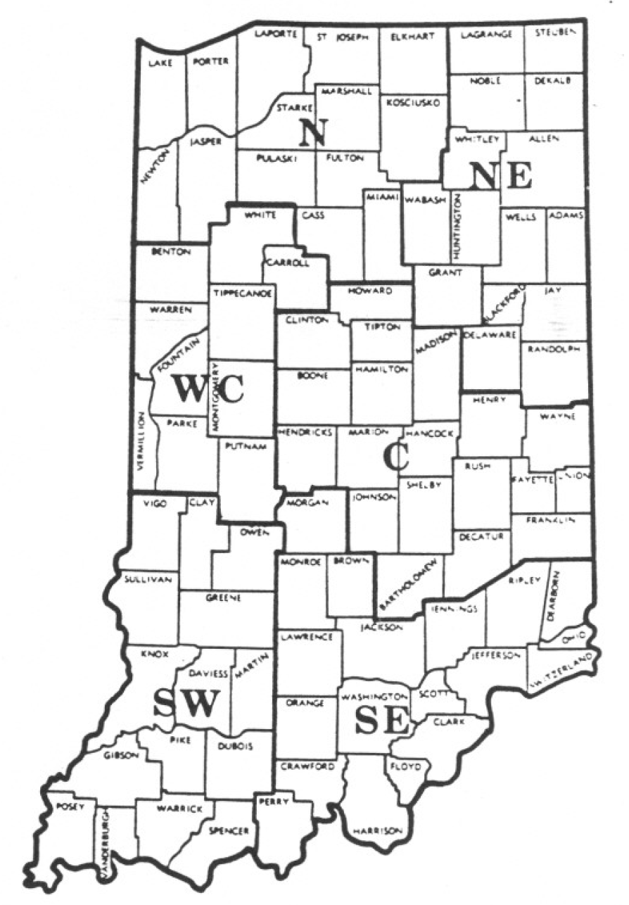
Figure I. Geographic areas used in the 1980 land value survey, Purdue University, July 1980.
This year began for Indiana farm people with the economically disturbing news of the Russian grain embargo. Farm costs rose, interest rates went to unheard of levels, grain prices were nothing to shout about and hog prices dropped below production costs. Thus, it comes as no surprise that results of the Purdue Land Values Survey indicates a S.9% state-wide decrease in the value of average bare land. Perhaps the surprise is that the decline was not greater.
The 1980 Land Values Survey was made possible by the cooperation of 229 persons who are knowledgeable about land values and cash rents – operating and professional farm managers, appraisers, realtors and agricultural lenders representing banks, PCA ‘s, the Federal Land Bank, Fm. H.A. and insurance companies. They reported on nearly on nearly all counties in Indiana giving their estimates of cash rent and market value for top, average, and poor tillable bare land. They also estimated the corn yield which might be expected over several years on each of these classes of land. In addition to farm land, they estimated the value of land moving into nonfarm uses – factory locations, housing, shopping centers, etc.
The state was divided into six areas (Figure 1) based roughly on general soil associations. Within any area, land values in a specific county may vary considerably from the area average. Thus, in using estimates from the survey (especially dollar figures per acre) potential buyers and sellers of land should remember that nothing substitutes for a good knowledge of one’s local land market. Our figures are useful guidelines, but the value of a specific farm still must be adjusted for buildings, nontillable land. drainage, soil type, fertility, etc.
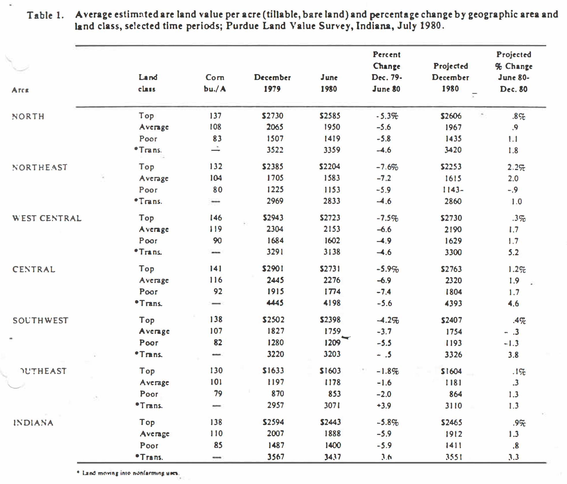
Table 1. Average estimated bare land value and percentage change per acre by geographic area and land class, selected time periods. Purdue Land Value Survey. Indiana, July 1980
One of the purposes of the survey is to obtain information on movements in land prices during the first half of the year (Dec. – June). While the average state-wide decline in tillable land values was just under 6%, declines in the two southern area, were less. For several years, land values in these areas have been stronger than in most other areas. and this relative strength continued in 1980. The northern area showed slightly less decline than the state average and the northeast. west central and central generally somewhat more. Declines in the last three areas were in the range of 4.9% to 7 .6% (Table 1).
Transitional land, that moving into nonagricultural uses. declined Jess than tillable land, 3.6% statewide. As in the case of tillable land, transitional land values were stronger in the two southern areas than elsewhere in the state. In the southeast, this land actually showed an increase of 3.5% from December to June.
The highest priced land usually has been reported in the west central area, but in 1980 this honor went to the central area – $2731 per acre for land with an estimated yield expectation of 141 bushels.
Statewide, land values in June 1980 were just about the- same as a year earlier. All three classes of land were down from a year ago in the northeast but were up slightly in the north and west central. The other areas had both ups and downs which roughly average out to no change.
Land values were fairly strong from June 1979 until about the end of the year. gaining around 7% statewide. But practically all this gain was lost from January to June 1980.
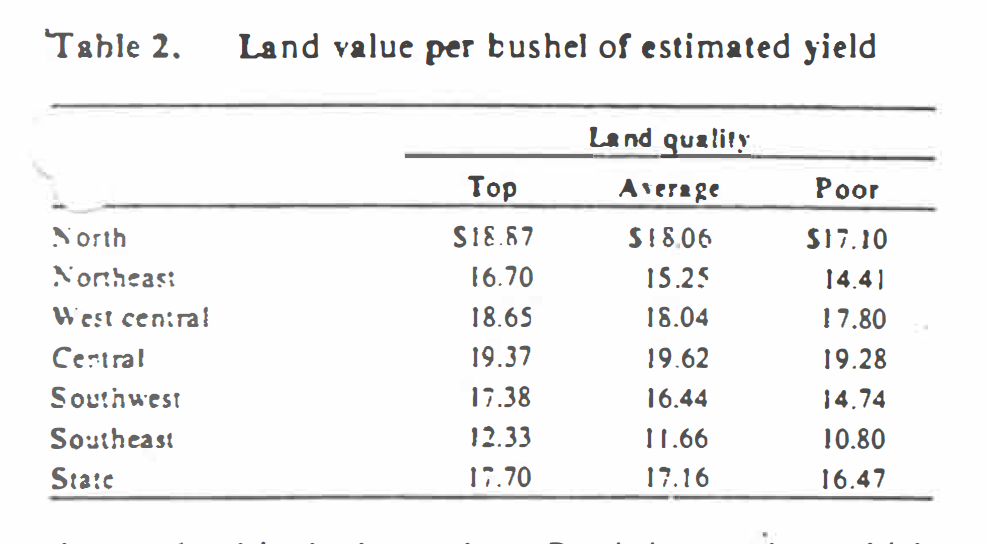
Table 2. Land value per bushel of estimated yield
Land Value per Unit of Production
A helpful “thumb rule” in evaluating different qualities of crop land is the land value per bushel of average corn yield, or value per acre divided by estimated yield. (Of course, management levels affect actual yields, so yield estimates should be based on typical management levels).
This value per bushel has been increasing in recent years but tended to drop slightly in 1980.
Land values per bushel of estimated yield were highest in the central area (Table 2) but there was less than a dollar per bushel difference on top quality land in the central, west central, and northern areas. The highest per bushel figure $19.62 was for average. not top, land in the central area. In all other areas, land value per bushel declined as land quality (yield per acre) declined. This makes sense because machinery and labor costs do not change in proportion to yield in moving from one class of land to another. Thus, with top land in the central area valued at S19.37 per bushel and average land at $19.62 the top land is the better buy. But it is not clear which quality land is the better buy here the market value per bushel is higher on better land. Each buyer needs to analyze his own situation. To illustrate. let’s take the state average of the top and average land and look at costs and returns from the owner operator point of view. Some cost of production will be about the same per bushel on land of different quality – seed, fertilizer, drying, hauling, machine repair, storing, interest on operating capital. etc. (variable costs). Others will be about the same per acre of different quality land-machinery depreciation, taxes, interest, and insurance; herbicides and insecticides; and labor (fixed costs). Here’s an example:
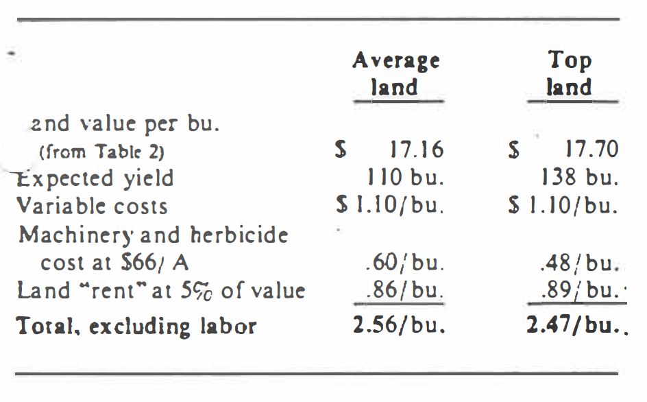
Table 2.1 Land value with expected cost
Top quality land, with a 9c per bushel lower production cost obviously is the better buy, if we have correctly separated fixed and variable costs. But costs per bushel tell only part of the story. If there is a positive profit margin to labor. the greater volume of production makes a big difference-possibly so big that production costs per bushel could be greater on the better land and it still would be the better buy, as indicated below:
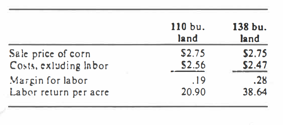
Table 2.2 Land value cost per 110-bushel and 138-bu.
The simple example illustrates the need to carefully analyze the returns from different classes of land to decide which is the relative “bargain.” And. it suggests that a buyer might press the upper side of the market for better land. The prospective buyer who estimates the annual land costs at around 5% of the market value of land (as in the example) obviously is expecting additional returns in the form of increasing land prices. And. the buyer who pays above the general market is bidding away some of the expected future gains arid may find himself owning land for several years which would not sell fur what he paid for it.
Land values per extra bushel of estimated yield, going from average to top land were in about the $21-22.00 range in the north. northeast. west central. and southwest: $18.20 in the central area and $14.66 in the southeast.
Average land value in each area was adjusted to 110 bushel yield (value of average land plus or minus the product of the value per extra bushel going from average to top land times the departure in the reported yields from 110 bushels) as follows:
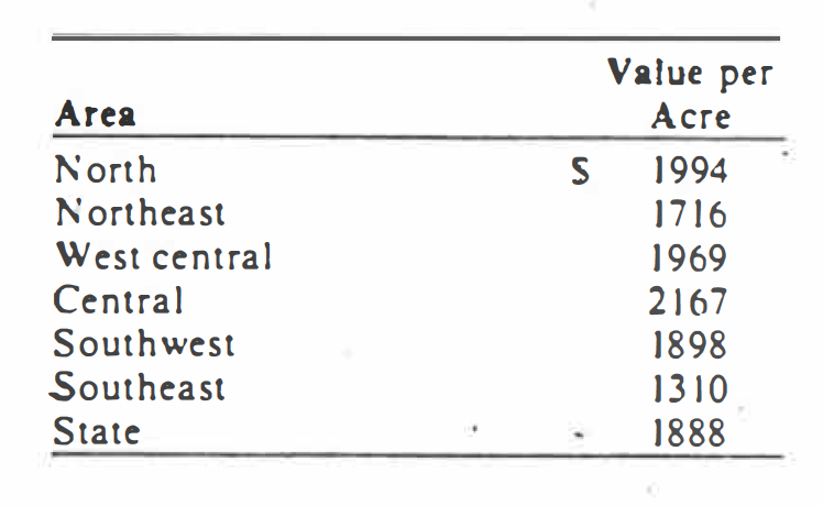
Table 2.3 Land value per 110-bushel by area
Note that central Indiana again shows up as a high priced area. Such factors as production costs, risk, markets, etc. probably cause some of the differences in prices between areas. But some of the differences are due to local demand, potential nonfarm use of land. etc. Farmers. particularly those just beginning might well look to the “bargain” areas to buy land. But they should look carefully for differences in production costs, risks and market-factors which may erase part or all of the advantage of lower land costs.
Cash Rent
Cash rents per tillable acre of bare land were up about 5% from 1979 levels for average land on a state-wide basis (Table 3). There was little or no change in the southern areas in top and average land rents. This may reflect spotty poor crop conditions in 1979. Higher 1980 rents for poor land in the southern parts of the state may have been due to the increase in profitability of the cow-calf enterprise. Increases in cash rent in the north and west central areas probably were due to a combination of good yields in 1979 and fairly good grain prices.
Cash rents per bushel of estimated yield approached $1 in the major grain producing area – central and west central. Rents for top and average land in the two southern areas were from 71 cents for 75 cents per bushel and from 82 cents to 91 cents in the north and northeast.
The same kind of analysis discussed above regarding the analysis of the profitability of buying different classes of land applies to renting land. Logically, a higher rent per bushel can be paid for higher yielding land. Fixed costs can be spread over more bushels on better quality land.
Cash rent as a percentage of June land value tended to be slightly higher than last year. State wide this increase was from about 4.8% in 1979 to 5% in 1980 (Table 3).
Farmers who are short on capital should consider the fact that they can cash rent more than 2 acres for the interest cost of buying 1 acre.
Outlook
So much for what we know about the recent past – what of the future? Survey respondents expect:
- A slight, almost insignificant, increase in land values by December 1980 (Table 1).
- A27% increase in land values by 1985, or about a 5% annual compound rate, about the same as last year’s estimates.
- Five-year average on farm prices of $3.01 for corn and $7.15 for beans. Last year their 5-year estimates were $2.83 and S7.40.
As has been the case in several recent years, the July/August period again appears critical in assessing the short-term outlook. As of this writing (mid-July), the specter of drought hangs over us. If the corn and bean crops are substantially reduced. those areas that have good yields (with high prices) may experience a sharp recovery in land prices while drought areas may see stable declining prices.
Over the longer run. world demand for farm products is increasing. new markets may open up for U.S. products, inflation will not be easily controlled and the security demand for land will continue (owners of land do not need to own gold!). Under these conditions, the 5-year estimates of land value increases of the respondents appear to me to be conservative.
Buying or holding land is. in some degree. an act of faith. As an economist. I believe that knowledge. study and analysis can help us make better decisions, but my basic philosophy is unchanged from the statement I made in this article a year ago.
“For the operating farmer who can profitably use additional land (perhaps spreading fixed costs over more acres or purchasing a base of operation), who can handle the cash flow requirements, and who can purchase near the “market price” with the expectation of 5 to 7 percent annual increase in value, investment in land at this time makes sense.” (There may even be some bargains’).”
Who, then, are the sellers of land? Those who do not depend upon land to use their labor and management and who have (1) better alternative investments or (2) need an increased cash flow. Even though they may expect increases in land values, what does it profit a man to gain the whole world by the time he dies and lose the joy of living? In other words, why live hard up and die rich?
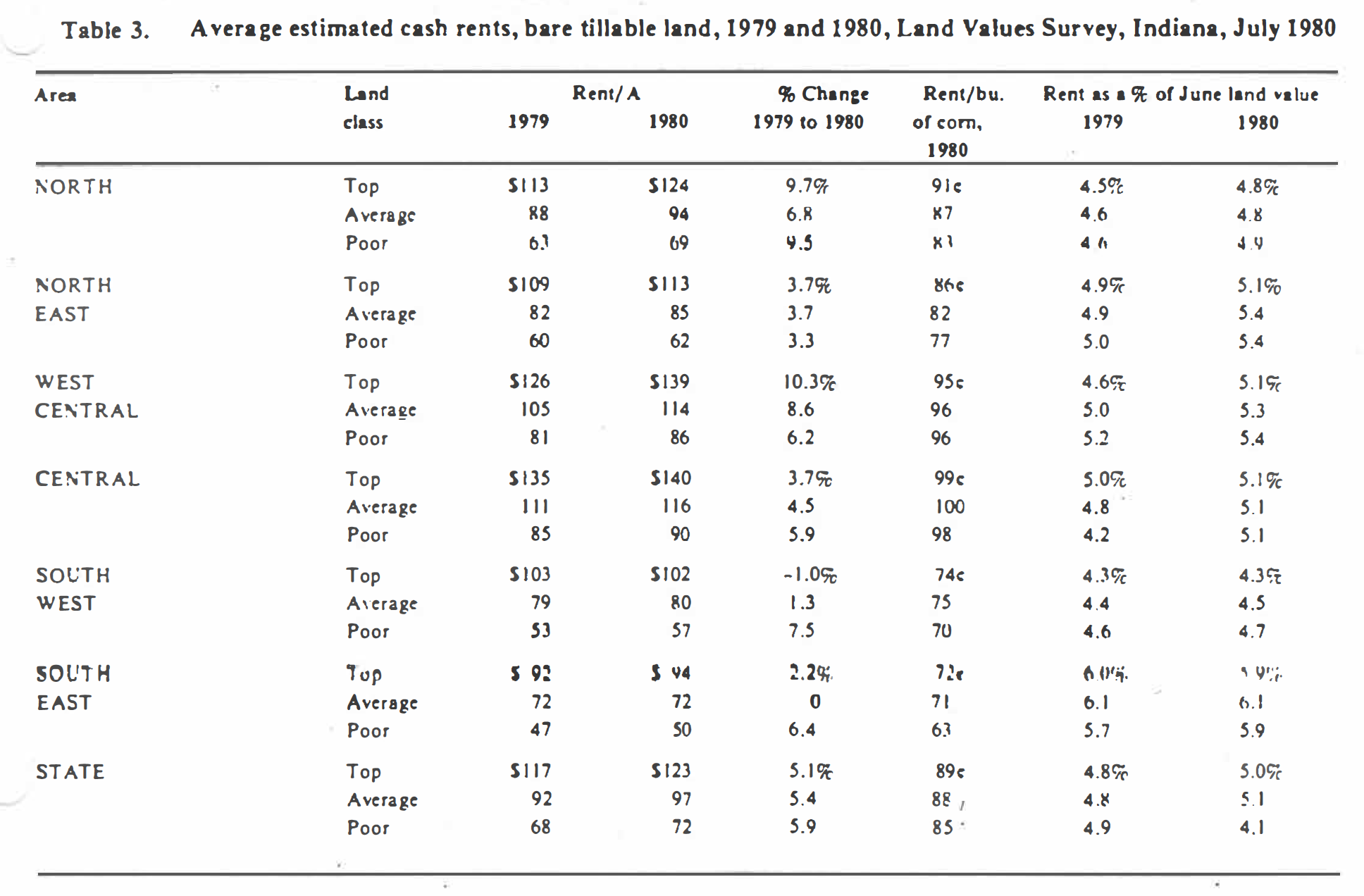
Table 3: Average estimated cash rents, bare tillable land, 1979 and 1980, Land Values Survey, Indiana, July 1980
![]()
![]()
![]()
![]()
![]()