Risk, Economic Value Added, and Capital Structure
May 13, 2003
PAER-2003-5
Michael Boehlje and Allan Gray
![]()
![]()
![]()
![]()
![]()
Most farm businesses use substantially less debt and less leverage than comparably sized non-farm and/or corporate businesses. Most farm term loans are structured with amortization schedules that result in a reduced indebtedness over time, whereas many non-farm businesses maintain a relatively constant indebtedness during their lifetime. And farmers appear to be highly motivated to reduce their indebted-ness and eventually be debt-free, whereas non-farm businesses appear less focused on this goal.
Why this bias against debt as part of the capital structure for most farm businesses? Isn’t it the case that debt is a source of risk, so reduced debt should be preferred? Is it an attempt to reduce cost, and is it the case that lower debt and less interest actually reduce cost? Should a farmer aspire to be debt free, or is there a desirable amount of debt that should be a permanent part of the farm business – an optimal capital structure? Are there some key concepts that might be useful in obtaining answers to these questions? This article discusses two concepts: 1) leverage and the principle of increasing risk, and 2) economic value added (EVA). These concepts are used to inform the decision of the preferred leverage ratio (optimal capital structure) for a farm business.
Financial Risk and Capital Structure
The risks that farmers face come from numerous sources, but their consequences can be categorized as affecting business operating performance or financial performance. Operating risk is commonly defined as the inherent uncertainty in the operating performance of the firm independent of the way it is financed. Thus, operating risk includes those sources of risk that would be present with 100 percent debt or 100 percent equity financing. Operating risk is evidenced by variability in the return on assets (ROA) of the business. The major sources of operating risk in any production period are price, cost, productivity, and production uncertainty. A number of factors may affect this variability over time, including weather, markets, technology, weed and insect pests, diseases, management practices, etc.
Financial risk or uncertainty is defined as the added variability of net returns to owner equity that results from the financial obligation associated with debt (or capital lease) financing. This risk results primarily from the use of debt as reflected by leverage; leverage multiplies the potential return or loss that will be generated with different levels of operating performance.
Financial risk is evidenced by variability in the return on equity (ROE) of the business.
There are other risks inherent in using debt. Uncertainty associated with the cost and availability of debt is reflected partly in fluctuations in interest rates for loans and partly through nonprice sources. Nonprice sources include differing loan limits, security requirements, and maturities, depending on the availability of loan funds over time. Thus, financial risk also includes uncertain interest rates and uncertain loan availability.
Principle of Increasing Risk Financial risk increases rapidly with the use of borrowed funds. The tendency for total risk to become greater at an increasing rate as the relative amount of nonequity (debt or capital lease) capital used in a business expands is referred to as the principle of increasing risk. The way this principle works is illustrated in Table 1.
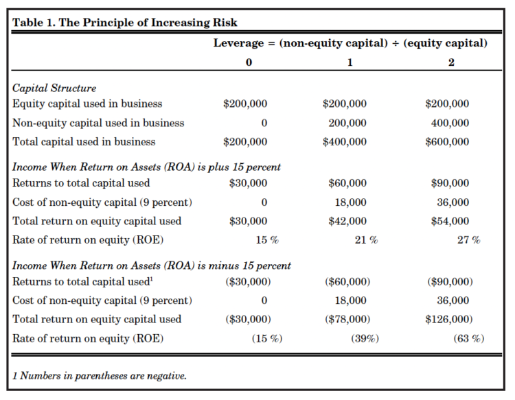
Table 1. The Principle of Increasing Risk
Assume a farmer has $200,000 of equity capital and can borrow additional capital at a cost of 9 percent. Consider first the situation where the operator has full equity in the business (leverage level 0 in Table 1). When a 15 percent return is earned on total assets (ROA), the gross return is $30,000; because there is no interest to pay, earnings are also$30,000 – a 15 percent rate of return on the $200,000 equity (ROE). Similarly, there is a 15 percent loss on owner equity under adverse business conditions (ROA equal to 15 percent).
In contrast, when the leverage level is 2, as reflected in the last column of Table 1, $400,000 of debt is combined with the $200,000 of equity to acquire $600,000 of assets. At a 15 percent rate of return on assets, returns to capital total $90,000, and after the interest cost of $36,000 (9 percent interest rate), returns to equity capital total $54,000, for a 27% rate of return on the $200,000 of equity capital. But when the rate of return on assets is negative 15 percent, the loss is $90,000, and the interest expense is $36,000, for a total loss of $126,000. This results in a very large rate of equity loss of minus 63 percent.
The numbers in Table 1 are graphed in Figure 1. Note the dramatic difference in the steepness of line A, which indicates the modest rate of increase in the ROE (assuming ROA is 15 percent and doesn’t change) as one increases leverage and debt utilization, compared to that of line B, which indicates the precipitous rate of decline in ROE (assuming ROA is minus15 percent and unchanged) as leverage and debt utilization is increased.
The use of nonequity capital –whether it is acquired by borrowing, leasing, or some other contractual agreement – creates a fixed financial commitment in the form of interest, lease payments, or other obligations. This commitment to the supplier of nonequity capital results in financial risk. As leverage (the amount of nonequity capital relative to equity capital) increases, the financial commitment increases; hence, the risk increases also. Note that with an equal percentage of gain or loss on assets (ROA), the magnitude and percentage of loss on equity capital (ROE) are greater than that of the gain. When ROA is positive 15 percent, the ROE for line A increases 12 percent as leverage approaches 70 percent, but when ROA is negative 15 percent the ROE is minus 48 percent as leverage approaches 70! Thus, we have the principle of increasing risk. At the same time, as long as the rate of return on capital invested (ROA) exceeds the cost of using nonequity capital, there is a gain from the use of leverage in the form of increased returns to the owner of the business.
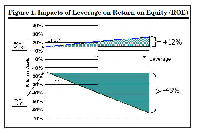
Figure 1. Impacts of Leverage on Return on Equity (ROE)
Risk Management and Leverage
The principle of increasing risk clearly indicates the potential disastrous financial consequences of more leverage – the potential loss with increased leverage is higher than the potential gain. Yet some firms safely use more debt and leverage than others. Are they just lucky, or is there an approach to borrowing that captures the benefits but reduces or mitigates the risk?
The answer is – yes, there is! Returning to the earlier discussion of business operating risk and financial risk, the total risk the firm faces can be managed by reducing either (or both). Buying insurance, hedging, diversification, and contract production are all approaches to managing operating risk. And if a firm can withstand only a given amount of total risk, it must more aggressively manage the operating risk as it borrows more and thus incurs more financial risk. The firm must balance operating and financial risk so as to not exceed the total risk-bearing capacity of the business. So the methods that more highly leveraged firms use to capture the upside potential of borrowing more, while protecting against downside risk exposure, are to give up some of that upside potential by, for example, buying crop insurance, hedging selling prices or, producing under contract. In essence, they incur some costs to reduce the operating risk in order to keep the financial risk within acceptable bounds. The implications of the principle of increasing risk are clear: if a business is going to use increased leverage, it must manage operating risk so as to limit total risk exposure.
Economic Value Added and Capital Structure
A concept critical in evaluating the performance of any business is economic value added. In generic terms, value added refers to the additional or incremental value created by an activity or a business venture. Economic value added is a refinement of this concept. It measures the economic rather than accounting profit created by a business after the cost of all resources, including both debt and equity capital, have been taken into account. Economic value added (EVA) is a financial measure of what economists sometimes refer to as “economic profit” or “economic rent.” The difference between economic profit and accounting profit is essentially the cost of equity capital. An accountant does not subtract a cost of equity capital in the computation of profit, so an accountant’s measure of income or profit is in essence the residual return to that equity capital since all other costs have been deducted from the revenue stream. In contrast, an economist charges for all resources in his computation of profit, including an opportunity cost for the equity capital invested in the business, so an economist’s definition and computation of the profit is net above the cost of all resources.
Sometimes this concept of profit is defined as pure profit or rent. In the terminology of a financial analyst, it is called “economic value added” or “EVA.” Thus, the fundamental concept of EVA is not whether the business or venture is profitable, but whether that profit is sufficient to compensate the equity capital invested in the firm at its opportunity cost and have any revenue remaining after compensating the cost of all resources. EVA essentially asks the question, is there any value created after invested capital has been compensated at a market determined required rate of return? In essence, a firm can report a positive net income according to GAAP (Generally Accepted Accounting Procedures) rules and legitimately report to the public that it was “profitable” by typical financial and business terminology and standards, but have a negative economic value added if that accounting profit is inadequate to compensate the equity capital at its required rate of return. The end result in this case is that even profitable firms do not always create value unless they earn enough to cover the cost of debt as well as the opportunity cost of equity capital.
Over time, a firm that consistently exhibits a negative EVA will be shunned by investors because it is not generating an adequate return to compensate the equity capital contributors, and they will move their funds elsewhere.
Computing EVA
The mechanics of computing EVA are relatively straightforward, as reflected in Table 2. Note that, as in the traditional computation of earnings, interest on debt capital is subtracted from operating earnings (earnings before interest and taxes –EBIT) to obtain net income. Then, an opportunity cost on equity capital is subtracted to obtain EVA. The opportunity cost on equity capital is computed as the equity or net worth of the business times a rate of return that reflects the rate required by investors in the business. This required rate is in reality an opportunity cost measured by the rate of return that could be obtained on equity funds if they were invested elsewhere. A positive EVA means the firm is generating a return to invested capital that exceeds the direct (i.e., interest) and opportunity cost of that invested capital; a negative EVA means that the firm did not generate a sufficient return to cover the cost of its debt and equity capital.
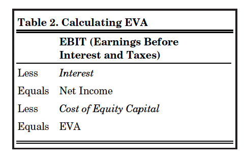
Table 2. Calculating EVA
Improving EVA
What insight does EVA provide about financial performance of a business and how to improve it? First, like any financial measure, the trend may be more valuable than the absolute value of EVA. Even if EVA is positive, a declining EVA suggests that financial performance is deteriorating over time and if this trend continues, EVA will become negative and financial performance unacceptable. A negative EVA indicates that the firm is not compensating its capital resources adequately and that corrective action should be considered if this negative EVA persists over time.
What are some corrective actions? First, operating performance with respect to operating profit margins or asset turnover ratios could be improved to generate more revenue without using more capital. Second, the capital invested in the business might be reduced by selling
under-utilized assets. This strategy will simultaneously improve operating performance through a higher asset turnover ratio, and reduce the capital charge against those earnings because of the reduced debt or equity capital investment. Third, redeploy the capital invested to projects and activities that have higher operating performance than the current projects or investments are exhibit-ing. And fourth, if the business is not highly leveraged, and the interest rate is lower than the required return to equity, change the capital structure over time by using debt as the primary source of funds to expand or grow the business. Even though this last strategy may increase interest cost, it will improve the EVA because a larger portion of lower cost debt and a smaller proportion of higher cost equity are being used to finance the business.
An Illustration
Let’s use these concepts to evaluate the implications of different capital structures for a case farm – MBC Farms. The cost of debt (the interest rate) for this farm is 8.8 percent, and the cost of equity, which reflects the opportunity cost of investing the equity elsewhere, is 10 percent. Panel A of Table 3 indicates the ROE and EVA for this farm for different combinations of operating performance (ROA) and capital structure (debt to total assets). Panel B of Table 3 illustrates the implications of implementing strategies to reduce operating risk (for example buying crop insurance or hedging/contracting selling prices) for the same combinations of operating performance and capital structure. It is assumed that the risk-reducing strategies incur costs of approximately $6,000 which reduces the ROA by .5 percent, but also reduces the downside risk in the ROA by 50 percent.
Note that in Panel A, when full exposure to operating risk exists, increasing the leverage (debt to asset) position from 23 percent to 70 percent results in a dramatic decline in ROE from 3.6 percent to -4.5 percent when the ROA is 4.8 percent. With an ROA of 4.8 percent, the EVA improves slightly from -$118,544 with 23 percent leverage to -$105,072 with 70 percent leverage. This improvement in EVA occurs because lower cost debt is being substituted for higher cost equity, and with a constant operating income, the substitution of less expensive for more expensive funding results in an improved EVA as debt utilization increases. It would appear that these two measures give different messages about financial performance in this situation; ROE declines as leverage increases, but EVA improves with increased debt utilization. In essence, even though the ROE is lower with higher leverage compared to lower leverage in this case, the value created is less negative because of the increased use of lower cost debt financing. Irrespective of whether overall performance of the firm is measured by ROE or EVA, performance is unacceptable, and when interest cost exceeds operating performance as measured by ROA, changing the capital structure does little or nothing to solve the problem.
With the average ROA of 9.52 percent, the ROE and EVA both increase modestly with increases in leverage. As ROA increases further to 14.28 percent, ROE increases dramatically from 15.9 percent with 23 percent leverage to 27.0 percent with 70 percent leverage. Note that the EVA increases only modestly compared to the ROE as leverage increases. This is a result of the fact that the cost of debt at 8.8 percent and the cost of equity at 10.0 percent are not widely different, and so the total capital charges for debt and equity used in computing the EVA do not vary dramatically in this case as leverage is increased.
Also note the additional information that EVA provides on financial performance for this business. When the ROA exceeds the interest cost, as it does with average returns and low debt (9.52 percent ROA and 8.8 percent interest), ROE (9.7 percent) exceeds ROA, which is an indication of acceptable performance. But EVA is negative in this case because the return to equity did not meet the cost of equity hurdle rate of 10 percent.
When costs are incurred to manage operating risk, as reflected in Panel B, the high and average ROA’s are reduced slightly, but the low ROA is increased from 4.8 percent to 7.14 percent. Consequently, the ROE’s and EVA’s for the higher level ROA’s are reduced only modestly from those of Panel A, and the impacts of increasing leverage are not changed significantly for the average and high ROA. But note the significant benefits of reducing operating risk for the low ROA level in terms of the ROE and EVA. Not only are the ROE and EVA generally higher, but the ROE in particular does not decline nearly as rapidly as leverage increases compared to the case of Panel A where operating risk is not reduced.
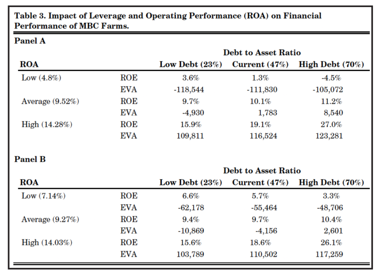
Table 3. Impact of Leverage and Operating Performance (ROA) on Financial Performance of MBC Farms.
So What?
The basic implications of this discussion are contrary to common practice in the financing of farm businesses. In general, the preferred capital structure for many businesses including farm businesses, involves some debt — assuming debt is a lower cost source of capital than equity. If debt is higher cost than equity, then a debt-free capital structure is preferred. Using increasing amounts of debt with a fixed equity base increases the financial risk of the business, but the best response to this increased risk is not always (or even often) to reduce debt use. Instead, the preferred response is to implement strategies to reduce the operating risk and thus the resulting financial risk that occurs with higher leverage and debt utilization. Such a strategy frequently results in a higher economic value added (EVA) and return on equity (ROE) without incurring unacceptable levels of risk.
![]()
![]()
![]()
![]()
![]()