Sources of Cycles in the United States Beef Industry
September 16, 1990
PAER-1990-12
Author: Kenneth A. Foster, Assistant Professor
![]()
![]()
![]()
![]()
![]()
Cycles in cattle numbers and price have been a fairly regular event throughout the current century. Most farmers are aware that, approximately every 10 to 12 years, prices reach a peak and begin to decline. One of the causes for the cyclical patterns is farmers’ tendency to base future production on current and recent past prices. For example, when prices are rising and profitable, expansion takes place. Expansion increases supply, which leads to lower prices in a subsequent period. Low prices and losses then create contraction in the industry and thus higher prices the next period. This dynamic process gives rise to the cattle production and price cycle. This paper deals with the source of persistence in cattle cycles and helps evaluate what determines both the length and the magnitude of the swings in production and prices.
The cattle cycle has a major influence on the financial status of the farm. Unfortunately, for the producers of feeder calves and finished cattle, the cycles in production and price run counter to each other. Thus, when prices are high, farmers in aggregate have fewer animals to sell. Conversely, when prices are low, farmers have larger numbers to sell. For a given supply schedule, the relative magnitude of the price and production swings are determined by the price elasticity of demand for the product. Historically, farm level demand for cattle has been fairly inelastic, leading to cycles characterized by a greater percentage change in prices relative to quantities. Large changes in price across the cycle result in increased financial uncertainty and greater risk for the farmer. Thus, the effect of cycles on the cattle industry relates to a broad set of concerns for farmers including marketing, finance, and management. Uncertainty about future prices helps to create the cyclical marketing and production dilemma, because many producers respond by using current prices as a forecast. As a result, financial burdens are often greatest when market conditions are at their worst.
Length of Cycle and Why Cycles Continue
A biological lag in production responses is the primary factor causing the cattle cycle to be longer than one or two years. When cow-calf operators make a decision to expand production, it requires the retention of heifers into the breeding herd. From the time this decision is made until an increase in cattle slaughter is noticed may be as long as three years. Add to this the psychological lag in making a decision to expand and the diversity of decision makers in the industry, and the expansion process may actually take five or six years to occur. Historical cycles have actually required about seven years on average for the expansion phase. The additional year may reflect a reluctance of producers to commit themselves to expansion until it is very clear that prices are truly rising.
An additional factor contributing to the persistence of the cattle cycle may be the fact that large numbers of heifers are brought into the herd during the expansion phases of the cycle. As this large pool of heifers age through the cycle, it causes a skewed age distribution. Then at some point late in the production cycle, it will be necessary to cull a greater number of cows to remove those heifers retained in the expansion. Replacing these aged cows creates a drain on the number of heifers available for slaughter and may contribute to the start of the next cycle. The research reported in this article examines both the biological lag and the skewed age distribution as explanations for the length and persistence of the cycles.
Two Models of Cattle Inventories
Two different approaches were developed to examine aggregate producer response to prices in the U.S. beef cattle industry. The first approach addresses the biological lag in production without any impact arising from the skewed age distribution. The second method allows for an inherent cyclical component in the replacement heifer retention due to the skewed age distribution over time. The two different relationships were then simulated along with a demand system for retail beef, fed cattle, and feeder calves. By comparing the results of these two models, we can isolate the impacts of the biological bag from the age distribution cyclical impacts and determine the potential for a cycle even when there is no built-in cyclical component in the supply response of producers.
Both models are based on annual data for the United States collected from Agricultural Statistics from 1965 to 1988. For further reference to the development of both approaches, any interested reader should refer to Foster.
Without a Cyclical Supply Component. This model of the beef breeding herd combined the replacement heifer and mature cow inventories. Doing so precluded evaluation of the effects of the age distribution, because it averages the culling rate across all ages of breeding animals. It was found that taking this approach resulted in a model with no cyclical supply component. Past prices were used in the analysis to both capture some of the psychological lag and because they represent the information farmers have available for decision making. The model also employed lagged values of the breeding herd to capture the biological lag in production response.
The short-run elasticity of the breeding herd with respect to a change in the feeder calf price was .019. That means that a one percent increase in the price of feeder calves will lead to a .019 percent increase in the size of the breeding herd the following year.
In a dynamic setting such as the one in which cattle cycles occur, a single period producer response to a feeder calf price change does not tell the entire story. The model also provides breeding herd responses for future years. These are presented in Table 1 under the biological lag only model.
* Notice, that the liquidation phase of the cycle should be expected to proceed more rapidly than the accumulation phase described. This is because there is no biological lag between the time the decision to scale down is made and the enactment of the policy.
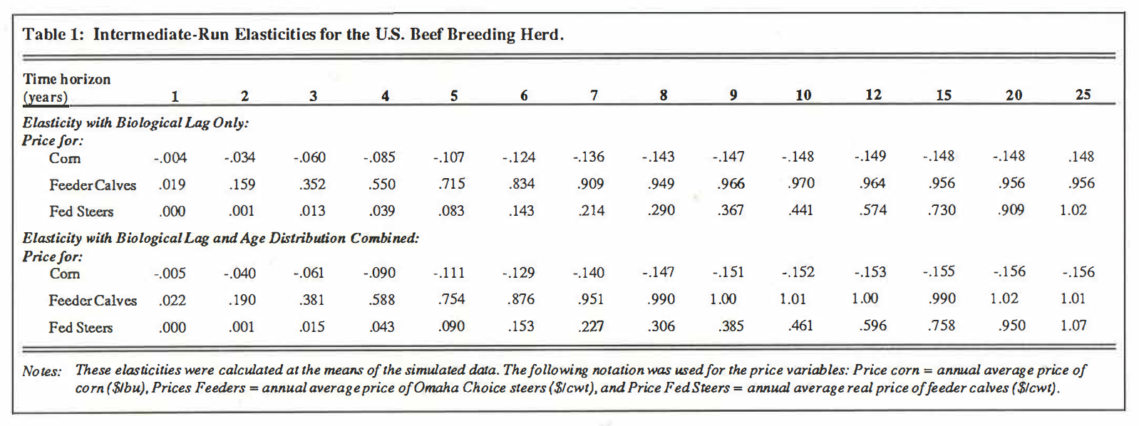
Table 1: Intermediate-Run Elasticities for the U.S. Beef Breeding Herd.
Notice that the elasticity for feeder price rises until the tenth year, then begins to fall. This means that producers continue to expand the breeding herd for the 10-year period and represents the completion of a cycle. However, these cycles are not long lasting. The elasticity levels off at a point where the herd size becomes stable. This means that, without any further intrusion on the industry, the initial shock from feeder prices will only last about two cycles and the impact during the second cycle will be almost imperceptible. The near equilibrium reached after one cycle is analogous to the point where the supply and demand schedules cross. Thus, this model suggests there would-be no longer-term affect causing a repeated cycle.
Also shown in the table are the elasticities for com and fed steer prices. The effects of the com price also appear to wear out after one cycle. The steer price, however, has a longer-term affect which arises from a trend implied by the price shock in the model of beef demand.
With a Cyclical Supply Component. The lack of a recurring cycle in the above model tells us that the separation of the age distribution may be an important component of the dynamic relationships in the cattle industry. Unfortunately, the USDA does not collect data specific to the age of cows. However, they do maintain data on the number of heifers kept for replacement and the number of mature cows. In this case, separate models were developed for mature cows and retained heifers. Proper specification of these allows the age distribution of the cows to be approximated from the retention of heifers in the past and an estimated annual culling rate of about 20 percent. The model for replacement heifers has a built- in cyclical component suggesting that there is in fact a response to the changing age distribution.
Separating mature cows and heifers has the added advantage of reducing some of the uncertainty with respect to the heifers. Some of the heifers counted as replacements will never enter the breeding herd. However, there is no accurate measure of this group. The assumption is that the percentage actually retained out of those counted as replacements will be rather constant from year to year. It would be dangerous to ignore the heifers completely because a sizeable portion will bear a calf, creating a potentially significant impact on the cattle market.
The elasticity measures derived from this approach are also in Table 1. They are listed under Biological Lag and Age Distribution Combined. This represents the percentage impact of a one percent change in the price variable on the sum of mature cows and replacement heifers. Notice that the cycles, resulting from feeder calf prices, are more long lasting than the previous set. The long run elasticities peak markedly every 10 years after the shock. This suggests a source of persistence in cattle cycles.
The elasticities implied by the two models are very similar. The primary differences are the recurrence of the cycle and slightly larger responses in the second approach.
Conclusion
The discussion above demonstrates how the combination of an inelastic demand curve for beef and the biological and psychological lags plus a skewed age distribution may result in a persistent cycle in the production and prices of cattle in the United States.
Cattle cycles are a well-documented phenomenon, but they are by no means exact or predictable. The models used in this study performed reasonably well in determining turning points in the size of the beef cattle breeding herd, but encompassed only two full cycles, both of which were atypical.
Producer responses to cattle cycles take three main forms. The first is the producer who responds to the prices in the marketplace and produces with the cycle. The second method attempts to hold production fairly constant over time to average the low and high prices. The third approach is to attempt to read the cycle and behave counter to it. Any of these approaches may be acceptable depending on the individual situation. Producers who are highly leveraged will find it difficult to sustain the losses, during low price periods, associated with the second and third strategies. However, good forecasters of future trends in cattle prices may be wise to gamble on the third strategy, which attempts to reduce their commitment during low price periods and boosts production when prices are high. However, the difficulty here is accurately determining the turning points. Inaccurate predictions may lead to production in conjunction with the cycle. One suggestion directly related to the results presented in this paper is for farmers to attempt to smooth out the age distribution of their breeding herd through their culling and retention practices. This will prevent them somewhat from being constrained to the cycle.
It was suggested earlier that the level of demand elasticity plays a significant role in determining the characteristics of the cattle cycle. Demand for beef has become more elastic since the mid-1970’s. In today’s economy, people are more willing to substitute other foods for beef when beef prices are relatively high. Thus, if there are no corresponding changes in the supply schedule, one would expect that in the future cattle price swings may be smaller relative to their accompanying quantity cycles. This will likely lead to more rapid expansion and contraction and slightly shorter cycles in the future. However, slow expansion to recent price increases suggests that the psychological lag may have lengthened, that is, the threshold price which producers view as sufficient to support expansion is higher now than in the past.
The importance of reflecting on cycles in the beef breeding herd is emphasized by their impact on the rest of the beef production chain. The number of cows and heifers available for breeding directly impacts the number of calves available to feedlots, and ultimately the amount of beef in the market. Both producers and packers need to be aware of the occurrence of these cycles and keep an eye on changes in the economic and political environment which might lengthen or shorten a cycle. By doing so, they may be more timely in adjusting their particular operation to ups and downs of the market.
References
Foster, K., A Dynamic Econometric Model of Inventories and Supply in the United States Bee/Cattle Industry, PhD Dissertation, University of California, Davis, California 1990.
USDA, Agricultural Statistics.
![]()
![]()
![]()
![]()
![]()