The New Method for Calculating Assessments Will Reduce Taxes for Farmland Owners
February 15, 2017
PAER-2017-01
Authors: Larry DeBoer, Professor of Agricultural Economics and Tamara Ogle, Community Development Regional Educator
![]()
![]()
![]()
![]()
![]()
Farmland assessments for property taxes rose rapidly from 2007 through 2015. The taxable assessed value of agricultural property increased by 81% statewide during these years, and as a result agricultural property taxes rose 63%. During this time property taxes for all taxpayers actually fell by 4%.
The reason for the farmland assessment and tax increase was an increase in the base rate of farmland. That’s the starting point for the assessment of farmland statewide. Increases in commodity prices and decreases in interest rates caused the base rate formula calculation to increase from $880 per acre in 2006 and 2007 to $2,050 in 2015, nearly a two-and-a-half-fold increase.
But in the legislative session of 2016, the Indiana General Assembly changed the base rate formula. This will stop the rise in the base rate and is projected to substantially reverse past increases. The base rate will fall 4% from $2,050 to $1,960 for taxes in 2017. Our projections show a further drop of at least 40% by the early 2020’s, to a base rate of $1,070. Farmland tax bills are likely to fall too.
This means, however, that tax bills of other taxpayers are likely to rise, and some local governments in rural areas are likely to see reductions in property tax revenue.
The Increase in Farmland Assessments, 2007- 2015
The story of the rising base rate has been told several times in the pages of the Purdue Agricultural Economics Report, most recently in June 2015. Here it is in brief.
The base rate is a dollar figure per acre calculated by the state’s Department of Local Government Finance (DLGF). All farm acreage in Indiana is assessed starting with this value. Each acre’s assessment is then multiplied by a soil productivity index, which measures the soil’s productivity for growing corn. The index varies from 0.5 to 1.28. Assessments for some acreage are then reduced by an influence factor, which is a percentage reduction based on factors that reduce productivity, such as forest cover or frequent flooding.
In most years from 2003 to 2015, the base rate was calculated using a capitalization formula, which divides the net income from an average acre by a rate of return. Net income is the average of rents on a typical acre and a calculation of operating income based on commodity prices, yields and costs. Starting in the mid-2000’s commodity prices began to rise. The corn prices used in the base rate formula rose from $2.00 in 2006 to $7.23 in 2013, and soybean prices rose from $5.78 in 2006 to $14.70 in 2013. The cash rent of an average acre, measured each year by the Department of Agricultural Economics land price survey, rose from $122 per acre in 2004 to $232 in 2014.
Just as important was the decrease in the rate of return in the denominator of the base rate formula. This rate is the average of the interest rates on farm real estate loans and farm operating loans, published by the Chicago Federal Reserve. The average dropped from 8.2% in 2006 to 4.7% in 2015. This reflected the general reduction in interest rates, partly the result of the Federal Reserve’s efforts to fight the Great Recession and encourage economic recovery.
The rise in rents and commodity prices in the numerator, combined with the fall in interest rates in the denominator, produced the rapid rise in the base rate. Farmland tax bills followed.
Table 1 shows the base rate calculation for taxes in 2014 and 2015. Since taxes in one year are based on assessed values from the year before, farmland taxes in 2014 were based on assessments for 2013. The base rate for 2014 taxes was calculated with six years of data, from 2005 to 2010. Capitalized values called “market value in use” were calculated by dividing cash rent and operating net incomes by the capitalization rate. Six years of calculations were made, the highest value was dropped, and the average of the remaining five was the base rate, rounded to the nearest $10.
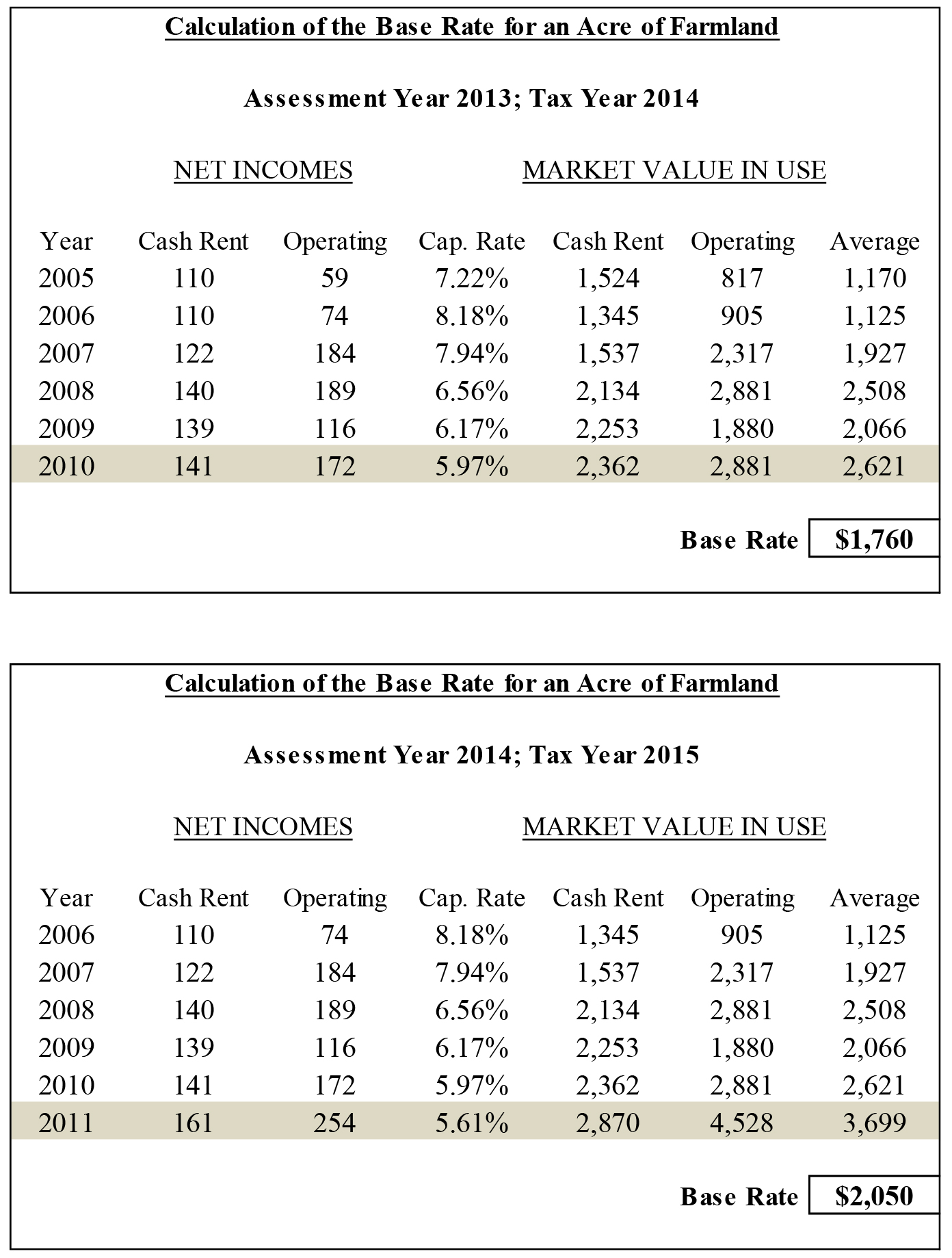
Table 1. Calculation of the Base Rate for Taxes in 2014 and 2015.
In 2015 the capitalized values for 2005 were eliminated from the calculation, and the values for 2011 were included. As it happened, the 2011 capitalized value was the highest of the six, so it was dropped from the average. The 2010 value had been dropped the year before, so it was included. In effect, the 2005 value of $1,170 exited the base rate average, and the 2010 value of $2,621 entered. The base rate rose 16.5% from $1,760 to $2,050.
The data used in the base rate calculation for 2015 taxes were for 2006 through 2011, so there was a 4-year lag between the latest year of data and the tax year. Cash rent increases continued through 2014, and commodity price increases continued through 2013. So, ever-higher values would have continued to enter the base rate formula—with the four-year lag—through 2018. Only in 2019 could the base rate have begun to decline. Projections showed the base rate topping $3,000 for 2018 taxes. Property tax bills would have continued to rise for five years after the downturn in farm incomes.
The General Assembly’s Response in 2016
The Indiana General Assembly passed a stop-gap bill in 2015, which froze the base rate at $2,050 for taxes in 2016. Without the freeze, it would have increased 18% to $2,420 under the existing formula. The 2015 bill limited increases after that. Hearings were held in the summer of 2015, and the result was included in Senate Bill 308, which passed by large margins at the end of the short session in March 2016. The governor signed it as Public Law 180. The bill included several property tax provisions, some more controversial than the change in farmland assessments.
SB 308 made two big changes in the base rate formula. First, it reduced the four-year lag to two, which is probably as small as the lag can be. Taxes in 2017 will be collected on the farmland assessments for 2016, which were set at the beginning of the year. Data from 2015 was the most recent available. Before, the base rate for taxes in 2017 would have been based on rents, prices, yields, costs and interest rates from 2008 through 2013. Now data from 2010 through 2015 will be used.
Second, the new formula introduces a system for adjusting capitalization rates, which splits the base rate calculation into two parts. The preliminary calculation uses the traditional capitalization formula, with a two- year lag instead of four. It uses the actual farm-related capitalization rates in the denominator. Then, the preliminary base rate is compared to the existing base rate certified by DLGF in the previous year. If the preliminary base rate is within 10% of the existing base rate, then the actual capitalization rates in the calculation would be replaced with 7% for all six years in the calculation. If the preliminary base rate was more than 10% lower than the existing base rate, a lower interest rate of 6% would be used. And, if the preliminary base rate was more than 10% higher than the existing base rate, a higher interest rate of 8% would be used.
This is intended to stabilize the base rate. If the preliminary calculation shows that the base rate will fall a lot, a low interest rate is used in the denominator to lessen the decrease. If the calculation shows a big rise in the base rate, a higher interest rate is used to lessen the increase. If the preliminary calculation comes close to the existing base rate, a middle-range interest rate is used to keep it there.
Table 2 shows the calculation for pay-2017. The first part of the table shows the preliminary calculation, and the second part shows the final calculation. The existing base rate for taxes in 2016 is $2,050. The preliminary calculation used actual interest rates and other data from 2010 through 2015—a two-year lag—and the result is $2,987. The preliminary rate is 45.7% higher than the existing rate, well above 10%. So, for the final calculation, all six of the actual interest rates are replaced with 8%. Since the actual interest rates ranged from 4.7% to 6.0%, the denominator of the calculation increases, which makes the final base rate smaller. The result of the calculation was $1,960, a 4% decrease from 2016’s $2,050 (and a 34% decrease from the preliminary base rate of $2,987).
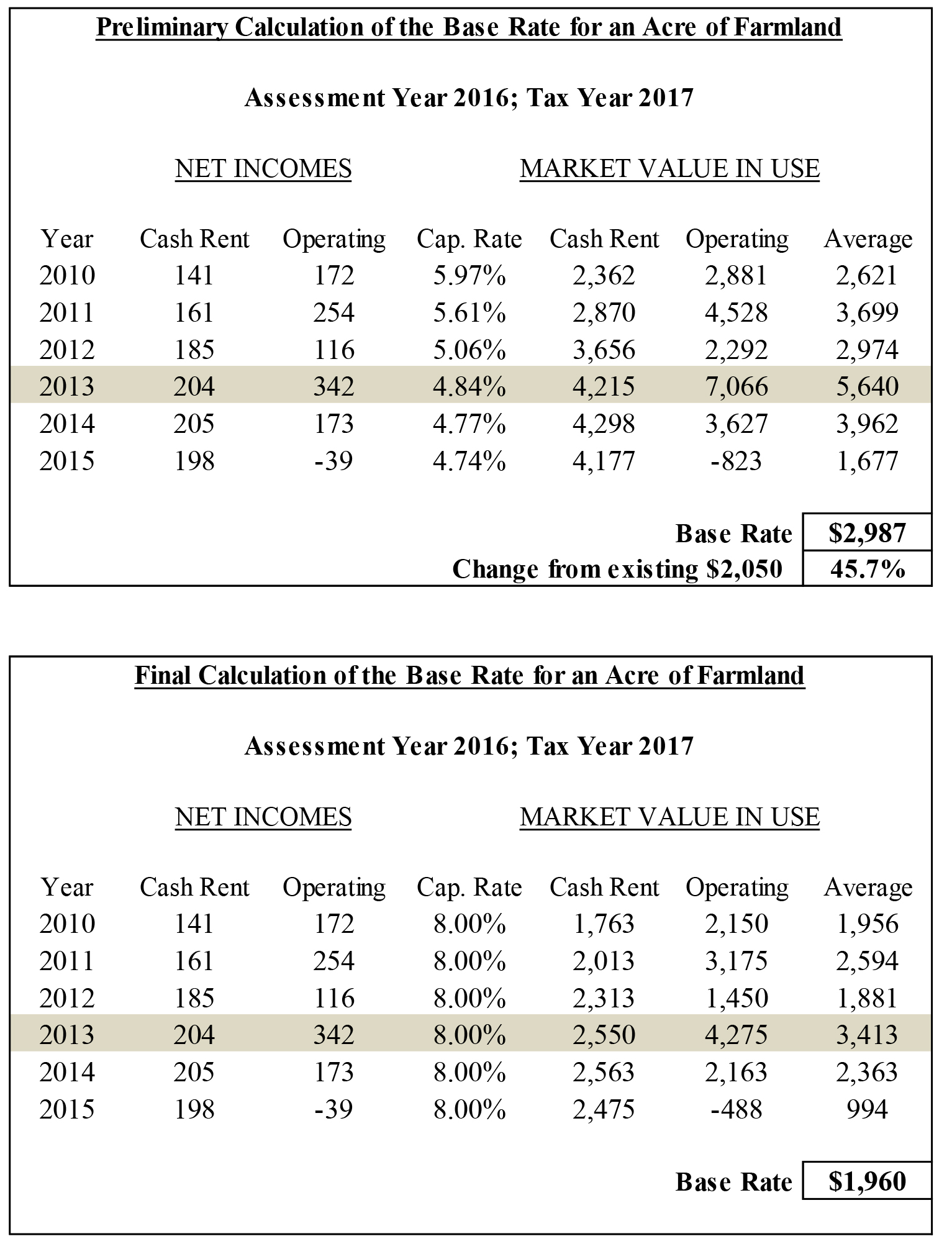
Table 2. Preliminary and Final Base Rate Calculation for Taxes in 2017.
Base Rate Projections to 2025
Projections of the base rate could be extremely accurate when the formula had a four-year data lag. For taxes in 2018, for example, the formula would have used data through 2014. Those numbers were already “in the books,” so they could be inserted into the existing formula to predict the 2018 base rate accurately.
Such precision is not possible now that the most current data are used in the calculation. The base rate for 2018 uses data for 2011 through 2016. The first five years are known; 2016 data must be projected (though many values are already clear). The projected base rate for 2019 uses data through 2017, so two forecast values must be included. The projected base rate for 2024 uses data for 2017 through 2022, so all of the data on commodity prices, rents, yields, costs and interest rates are forecasts.
The appendix describes the sources of our forecast data in detail. In general, prices settle near $4 per bushel of corn and $10 per bushel of soybeans by 2021 and after. Average cash rent falls to $179 per acre by 2025. Yields trend upward to 183 bushels per acre for corn and 55 bushels per acre for soybeans by 2025. Costs trend upward by about 2% per year. Interest rates rise to near 6.5% in 2022 and after.
Figure 1 shows projections of base rates using the old capitalization formula, the SB 308 calculation of the preliminary base rate, and the SB 308 final base rate. They are based on the best forecasts we could make about future corn and soybean prices, yields, costs, rents and interest rates. But another word for forecasts is “guesses.”
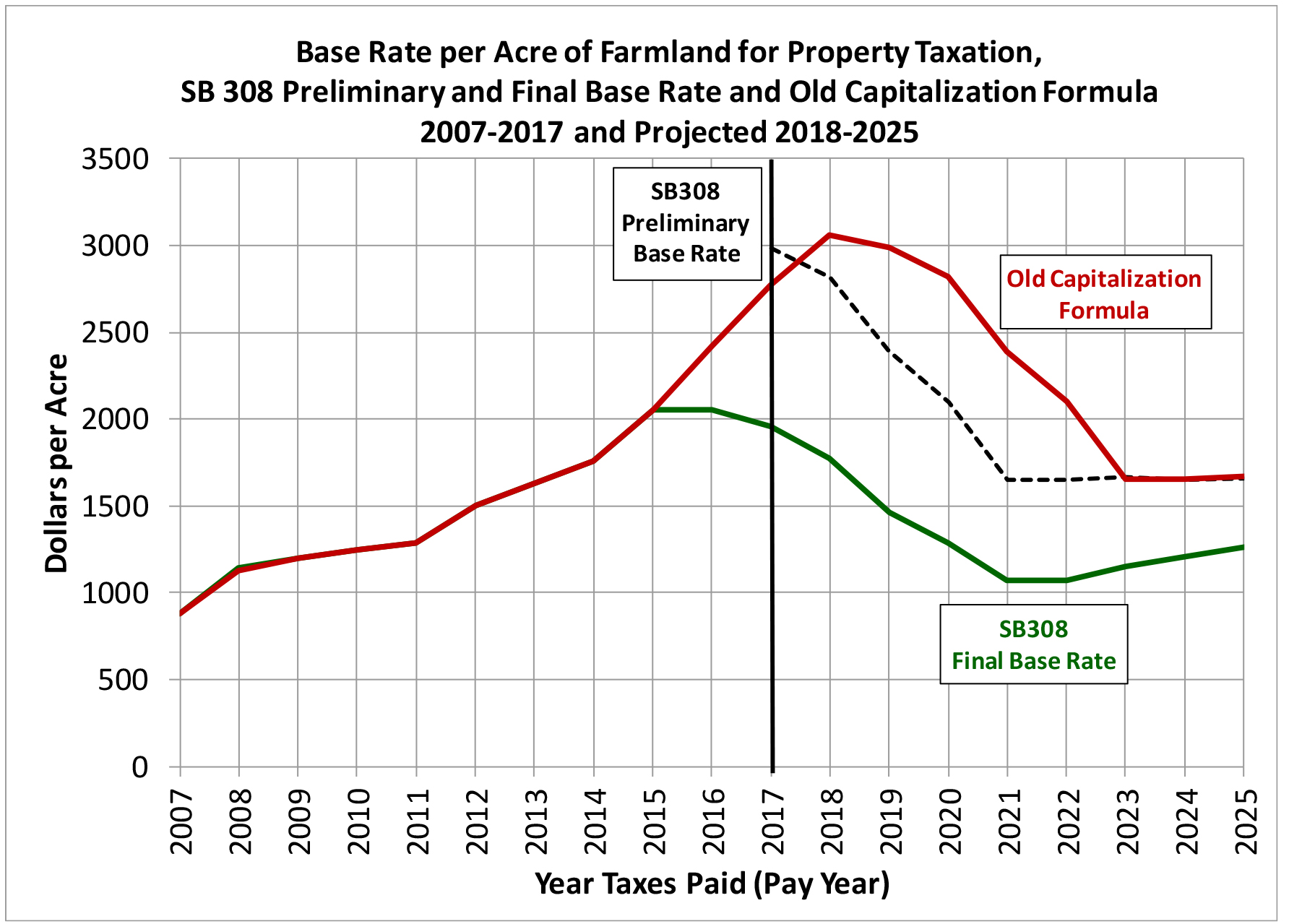
Figure 1.
The old capitalization formula used actual interest rates with a four-year data lag. Its value was projected to peak in 2018 at $3,065. Since that value was based on known data through 2014, it’s a very good guess. After 2018 lower commodity prices would have begun reducing the base rate under the old formula.
The dotted line is the preliminary base rate calculation under the new formula in SB308. It uses actual interest rates with a two-year lag, so it’s the same as the old capitalization formula, just two years early. That is, the preliminary base rate figure for 2017 is the same as the old capitalization formula base rate for 2019.
The 2017 preliminary base rate is $2,987, well above the 2016 base rate of $2,050. As a result, under the SB308 formula, the final base rate uses capitalization rates of 8% in the denominator for all six years of the calculation (see Table 2). Since the actual interest rates were lower than 8%, the final base rate is lower than the preliminary base rate. Base rate projections are shown in Table 3.
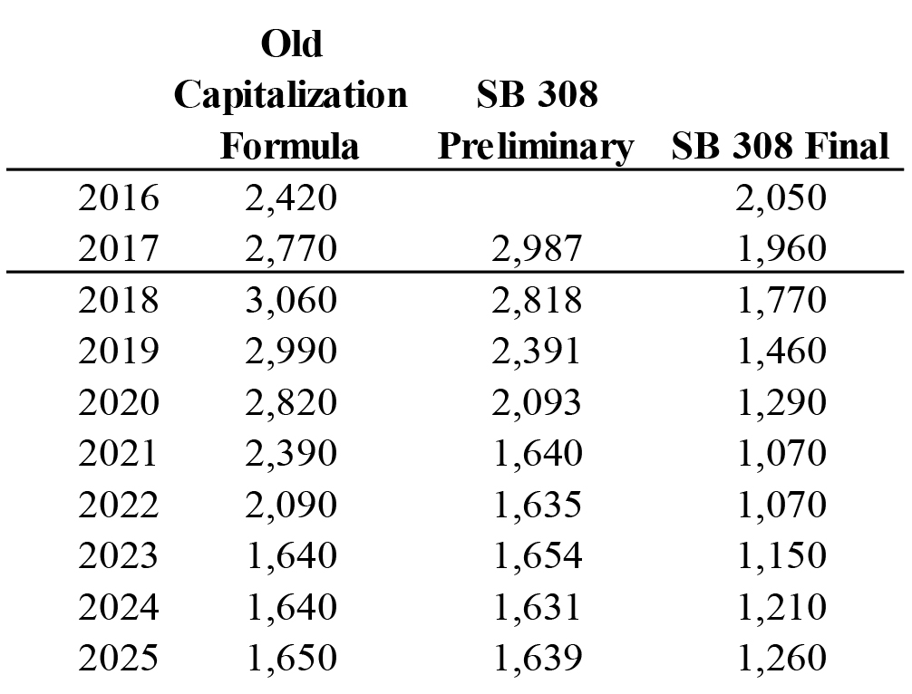
Table 3. Base Rate Projections, 2018-2025
The base rate is $2,050 for taxes in 2016, and the DLGF has announced a base rate of $1,960 for taxes in 2017. We project that under the SB 308 formula the base rate will continue to decline through 2021, to $1,070. This would be a 48% reduction from the current value. Reductions from the old capitalization formula are even larger. The SB 308 formula delivers tax relief to farm land owners compared to what would have been (the old capitalization formula) and compared to what exists now (the current base rate).
Effects on Taxpayers and Local Revenues
If farmland owners pay less in property taxes, either other taxpayers will pay more, or local governments will receive less revenue, or both. Local governments might charge higher property tax rates to raise the same revenue from lower taxable assessed value. Or, local governments might not raise tax rates enough to compensate for the drop in assessed value, so that revenue will be lower.
If tax rates go up, more taxpayers will see their tax bills exceed their property tax caps. They will receive tax cap credits to hold their tax bills at their caps. These credits are taxes that property owners do not pay, and revenue that local governments do not receive. Some local governments will collect a smaller share of their property tax levies.
If levies are not reduced, tax rate increases will be greatest where farmland is a larger share of taxable assessed value. In urban counties,
farmland is often a very small share of assessed value. The decline in the base rate would have little effect on tax rates. In rural counties, however, farmland can be a large share of taxable assessed value. Tax rates are likely to rise more in these rural counties.
The map in Figure 2 shows counties where tax rates are likely to rise most as a result of a 48% reduction in the base rate of farmland. This is the maximum projected drop in the base rate from the $2,050 value in 2016, projected to occur in 2021 and 2022. Projected tax rates are calculated simply by dividing the property tax levies of all local governments in a county by the county’s assessed value, less a 48% decline in farmland assessments. Many other rate, levy and assessment changes will affect tax rates in the next five years, but this map shows which counties are likely to be affected the most by the decline in the farmland base rate.
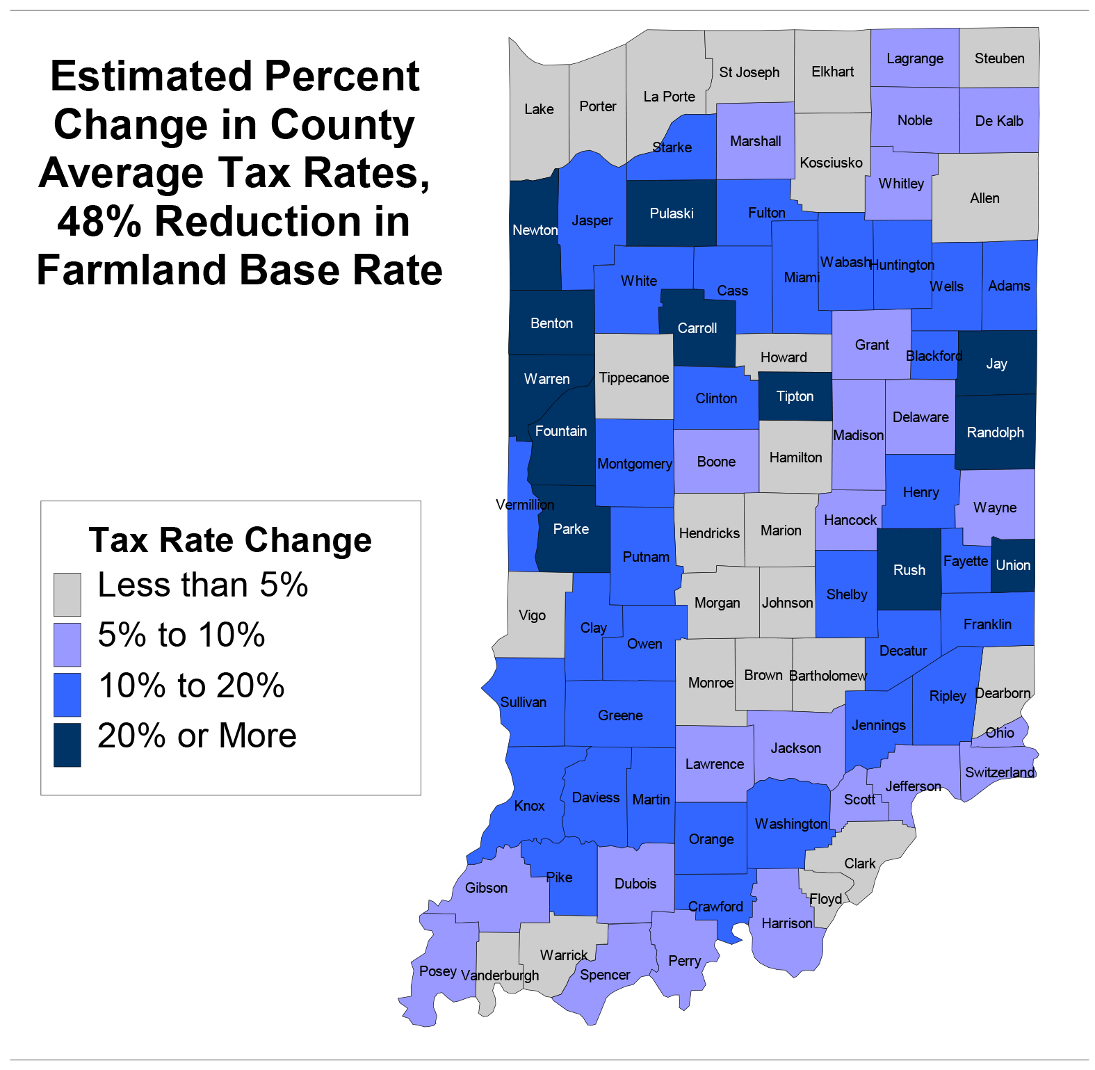
Figure 2.
There are a dozen rural counties where tax rates would increase by 20% or more in this exercise. These are counties where farmland is an especially large share of taxable assessed value. Farmland owners would pay these higher rates on their lower farmland assessments, which is why farmland tax bills will fall less than the base rate. The tax bills of rural homeowners and other property owners would reflect the full increase in the tax rate.
Local governments will collect a smaller share of their property tax revenue if higher tax rates push more taxpayers above their tax caps. However, in many rural counties outside of cities or towns, tax rates are well under $2.00 per $100 assessed value, which means only the most expensive houses are above their tax caps. Increases in tax rates would increase the tax bills of property owners, but most would remain under their caps and so would pay their full tax bills.
In cities and towns in rural areas, tax rates are often above $2, because the city or town rate is added to the county, township and school rates. There is usually not much farmland in these cities or towns, of course, but the county and school rates that city or town taxpayers pay would increase, pushing more of them above their caps. Rural local governments that overlap cities or towns would be most likely to lose revenue to the tax caps, as a result of the decrease in the farmland base rate.
Is SB 308 a Tax Cut for Farmers or Tax Bill Stabilization?
While we chose the best forecasts of commodity prices, rents, yields, costs and interest rates that we could find, they will be wrong. All forecasts are. How much will these errors affect the projected base rate of farmland? Table 4 shows the results of 14 alternate simulations to find out.
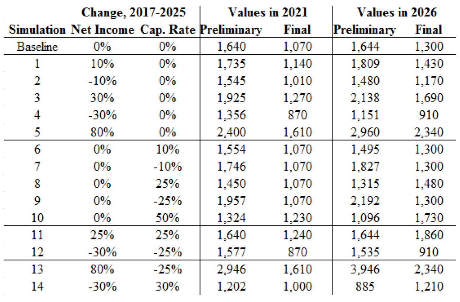
Table 4. Alternate Base Rate Projections.
The table shows variations in the preliminary base rate numerator, which is net income, and the denominator, the capitalization rate, for all forecast years 2017-2025. Simulation 11, for example, shows results if both net income and the capitalization rate are 25% higher than the forecasts used for the projections shown in Table 3 (which is the “baseline” projection in Table 4). The projected preliminary and final base rates are shown for two years, 2021 and 2026. The year 2021 is five years in the future. The base rate calculation will use data for 2014 through 2019. Data for 2014 and 2015 are already known, while data for 2016 through 2019 are forecasts.
The year 2026 is ten years hence, and is based on forecast data for 2019 through 2024.
The results of variation in the forecasts of net income are shown in simulations 1 through 5. In every case the preliminary values for 2021 and 2026 remain well above the final values, an indication that the 8% capitalization rate is used in the denominator of the final calculation. With the denominator constant, the final base rates vary in proportion to net income. The two known values are fixed for the base rate in 2021, so (for example) a 10% increase in net income results in a 6.5% increase in the final base rate. In 2026 all six years of data are forecasts, so a 10% increase in all six net income figures results in a 10% increase in the base rate.
Variations of plus or minus 10% are minor changes. The 30% changes are consistent with the typical variations that occurred during the 1995-2015 period. Net income 30% below the baseline is consistent with the worst net income years in the past 20. The final base rate is $870 for 2021 and $910 for 2026 in that case. Net incomes that are 80% above the baseline are consistent with the best years in the past 20—the 2007 to 2014 period. The 2021 final base rate is $1,610, and the 2026 rate is $2,340. Remember that these percentage variations are sustained changes over ten years. Single years of high or low prices or yields would not produce such large differences from the baseline.
Simulations 6 through 10 show the effects of variations in the capitalization rate, which in our projections are based on the 10- year Treasury bond yield forecast by the Congressional Budget Office (CBO), plus a premium (see the appendix for an explanation). Variations within 25% have no effect on the final base rate for 2021. The projection remains at $1,070. This is because in each case the preliminary calculation remains more than 10% above the previous year’s base rate, so the final calculation uses an 8% capitalization rate in all four simulations.
The final base rate for 2026 changes only in simulation 8. The capitalization rate rises to 8.1%, which drops the preliminary value below the previous year’s base rate. The calculation uses 7% as the final capitalization rate, so the final base rate is higher. This is near the result from projections made in 2015, when the CBO’s long run interest rate forecasts were higher. Simulation 10 shows the results of an increase in the capitalization rates to near 10%, similar to those from the late-1990s. The preliminary value is higher than the previous year’s base rate in each case, so the final capitalization rate is 7% in 2021 and 6% in 2026. The final base rate is higher than the baseline.
Simulations 11 and 12 combine changes in net income and the capitalization rate to show results for an expanding economy and a depressed economy. If both the general and farm economies expand faster than the baseline forecast, commodity prices and interest rates should be higher. Final base rates increase from baseline values. If the economy is depressed compared to baseline, commodity prices and interest rates should be lower. Final base rates decrease from the baseline values.
The base rate is $2,050 for pay-2016. It will be $1,960 for pay-2017. In all 12 of these simulations, ranging from minor to extreme differences from our baseline, the final base rates in 2021 are much lower than the current base rate. The final base rates in 2026 are lower than current base rate in 11 of the 12 simulations. There can be little doubt that the new base rate formula in SB 308 will mean a tax cut for farmland owners.
Finally, simulations 13 and 14 look at extremes. Simulation 13 has net incomes that match the highest sustained values and capitalization rates that match the lowest sustained rates over the past 20 years. The old capitalization formula would have resulted in base rates peaking at $3,065 with these values (see Figure 1). The SB 308 formula results in a base rate of $2,340 by 2026.
Simulation 14 is based on lower net incomes and higher capitalization rates that produce a preliminary base rate of $885 in 2026. That’s near the lowest base rate that ever resulted from the old capitalization formula ($880 in 2006-7). The SB 308 calculation results in a higher final base rate of $1,210 for 2026.
Under these conditions the old capitalization formula produced base rates ranging from $880 to $3,065. The new formula projects base rates ranging from $1,210 to $2,340. The new formula stabilizes the base rate in extreme conditions.
So, what is this new base rate formula? There’s hardly a doubt that it will reduce farmland base rates substantially over the next five years and beyond. It’s a tax cut for farmers.
But Indiana’s Supreme Court requires property assessments to be based on objective measures of property wealth. While it was never tested in court, the old method used objective data in a capitalization formula, which is one of the recognized methods for measuring wealth. Arbitrary changes in assessment methods to deliver tax cuts to particular property owners may not be Constitutional under the court’s standard.
It might be argued that the new legislated limits on capitalization rates are simply stabilizing, as demonstrated in simulations 13 and 14. Extreme base rate values are limited, but perhaps farmland owners will pay the same taxes, averaged over the long run. The legislated capitalization rates of 6%, 7% and 8% appear to be based on past variations in interest rates. If future interest rates vary around this legislated range, then the stabilization view will be strengthened. If future interest rates remain lower than this range, then SB 308 will look more like an arbitrary tax cut for farmers.
Appendix: Methods and Sources for Base Rate Projections
Estimates for Corn and Bean Prices, Yields and Variable Costs: For the projection of the farmland base rate using the capitalization formula we used long-term forecasts from the University of Missouri’s Food and Agricultural Policy Research Institute (FAPRI) publication, U.S. Baseline Briefing Book: Projections for Agricultural and Biofuel Markets, (March 2016) as well as FAPRI’s April Update. The publication includes forecasts for price, yield, variable costs, and government payments by crop from crop year 2015/2016 to crop year 2025/2026. These figures for corn and soybean prices were used in the capitalization formula. Variable costs and yields were adjusted for Indiana by calculating the percentage difference between historical Indiana and national values, averaging the percentage difference and using that average to adjust FAPRI’s forecasts.
Estimates for Government Payments: There are two basic alternative government payment programs for farmers: Average Revenue Coverage and Price Loss Coverage. FAPRI reports the adoption rate through the end of our current Farm Bill and forecasts an adoption rate after that as well as forecasting payments for both corn and soybeans through 2025 crop year. A weighted average based on the adoption rate of the two different programs was calculated for both corn and soybeans each year to estimate the government payments received for the capitalization formula. The corn and soybean average payments were then averaged to come up with an average total government payment per acre for the given year.
Overhead Costs: In this year’s Purdue Crop Cost and Return Guide, the estimation of overhead costs outside of property taxes increased only .5% over the figure DLGF used last year. With pressure from lower crop prices we expect farmers to keep overhead costs for machinery and family labor from growing at a high rate. For this forecast we assumed a 1.5% growth rate in the overhead costs through 2026.
Cash Rent: The cash rent number used in the capitalization formula is the average cash rent for the state as reported by the Purdue Land Value and Cash Rent Survey less DLGF’s estimate of the average property taxes per acre. To come up with this value we projected rent and average property tax separately.
For cash rent, we used Michael Langemeier’s (Purdue Ag Econ Department) projections for a west central Indiana farm taking the projected change in the west central Indiana cash rent and applying it to the state average.
Based on a 6-year average dropping the highest value of property tax as a percentage of the base rate, property taxes were forecast at 1.53% of the base rate for taxes paid in a particular year. The forecasted cash rent less this property tax estimation was used in the capitalization formula.
Capitalization Rate: The capitalization rate used in the farmland assessment formula is the average of the farm real estate and farm operating interest rates. This capitalization rate is closely correlated with the ten-year Treasury bond yields. In August 2016 the Congressional Budget Office projected that the ten- year Treasury rate will rise to a long-term level of 3.6% by 2022. The farmland capitalization rate averaged 2.9 percentage points above the 10-year Treasury between 1995 and 2015. We assume that the farm capitalization rate will rise to 6.5% by 2022, which is the CBO’s 10-year Treasury yield projection plus 2.9%.
![]()
![]()
![]()
![]()
![]()