


Stress Testing Financial Performance

Stress testing describes a range of techniques that can be used to access the vulnerability of a firm’s balance sheet and income statement to changes in prices, production, or financing. Stress testing can be an extremely useful tool when evaluating strategies for dealing with lower prices, higher costs, asset purchases, and changes in loan terms. In this article, a case farm in west central Indiana is used to examine the impact of a decline in gross revenue, and the purchase of additional machinery and equipment on key financial ratios.
Before examining the gross revenue and asset purchase scenarios, let’s briefly examine 2015 financial performance for the case farm, and baseline projections for 2016. The case farm has 3000 acres of corn and soybeans. Of the 3000 acres operated by the farm, 2250 acres are cash rented from several landlords and 750 acres are owned. The first column in table 1 contains financial performance information for the case farm in 2015. Wet conditions hampered corn yields in 2015, and contributed to the negative net farm income. It is also important to note that the farm replaced a combine in 2015. The second column in table 1 contains baseline projections of financial performance for 2016. Trends yields and futures prices were used to develop the revenue projections. Fertilizer costs and cash rent were projected to be lower in 2016. The case farm plans on replacing one of its tractors in 2016. Net farm income, though relatively low compared to net farm income from 2007 to 2013, is projected to be approximately $48,000 in 2016. Land values were assumed to decline 5 percent in 2016.
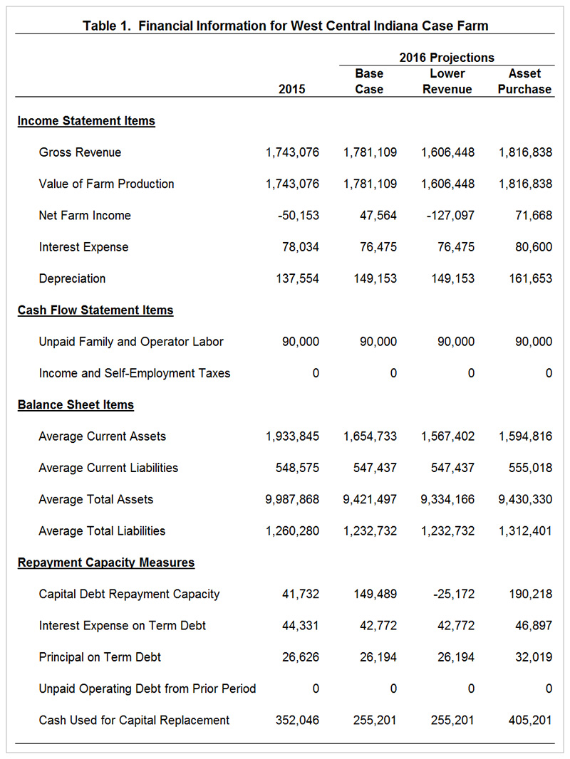
The third and fourth columns present financial information for the decline in gross revenue and asset purchase scenarios. The decline in gross revenue scenario assumes that corn and soybean prices for the 2016 crop will be 10 percent lower than the current futures prices. The crop prices for the 2015 crop to be sold in early 2016 were not changed. Comparing the second and third columns, the decline in crop prices has a large negative impact on net farm income. For this scenario, net farm income is projected to be a negative $127,000. The decline in revenue pulls down working capital and creates repayment capacity problems. The asset purchase scenario (i.e., purchase of a soybean planter) assumes a 5 percent increase in soybean yields, a $5,000 reduction in repairs, and a $12,500 increase in depreciation. The new planter is assumed to cost $150,000. One-half of the funds needed for the planter is assumed to be borrowed via an intermediate term loan. Cash is used to cover the remaining funds needed for the planter. Net farm income for this scenario is projected to be approximately $72,000. It is important to note that working capital declined under this scenario.
The financial information in table 1 was used to compute the key financial ratios illustrated in table 2. For definitions and discussion of key financial ratios, see the following articles (here, here, and here). We will first compare the 2015 ratios to the 2016 baseline projections (i.e., base case). Though still strong, liquidity deteriorates in 2016. Specifically, working capital per acre declines $93. The debt to asset ratio is projected to increase slightly in 2016. The asset turnover ratio is computed by dividing value of farm production by average total assets. The projected increase in the asset turnover ratio in 2016 is the consequence of a relatively higher projected gross revenue and the decline in land values. The operating profit margin is computed by dividing net farm income plus interest expense minus family and operator labor by value of farm production. The higher projected net farm income in 2016 results in an increase in the operating profit margin. The term debt coverage ratio measures the farm’s ability to cover principal and interest payments on term debt. A ratio above one indicates that these term debt payments can be covered. The replacement margin coverage ratio measures the farm’s ability to cover principal and interest payments on term debt, and replace capital assets such as machinery and equipment. A ratio above one indicates that these items can be covered. The case farm appears to be able to cover principal and interest payments in 2016, but is going to have trouble replacing assets. To make the asset purchases under the 2016 baseline projections, the case farm has to draw down working capital.
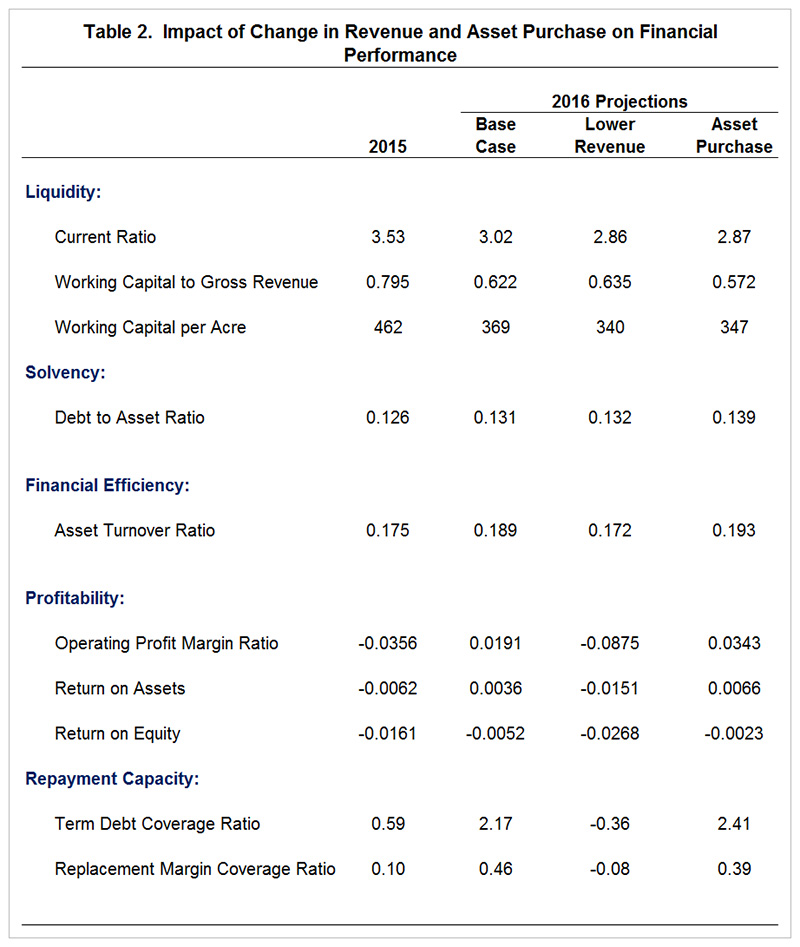
The third column (lower revenue column) in table 1 illustrates the impact of a 10 percent decline in corn and soybean prices for the 2016 crop. Liquidity and solvency are still relatively strong for this scenario indicating that it will take more than one year of low gross revenue for these measures to weaken markedly. However, it is important to note that compared to the baseline projections working capital per acre declined another $29. Financial efficiency, profitability, and repayment capacity declined substantially under this scenario. The asset turnover ratio dropped from 0.189 to 0.172. The operating profit margin, return on assets, and return on equity are all negative under this scenario. Further, repayment capacity is now worrisome. To cover principal and interest payments on term debt, the farm will need to draw down working capital. If this scenario plays out, the case farm will need to scrutinize their marketing strategies and look for ways to cut costs without dramatically impacting crop yields.
The fourth column (asset purchase column) examines the impact of purchasing $150,000 in machinery and equipment. One-half of the asset purchase was assumed to be borrowed. Under this scenario, gross revenue is the same as it was under the base case scenario. Due to the expected positive impact on soybean yields, the asset purchase resulted in an increase in profitability when compared to the baseline projections. Liquidity, solvency, financial efficiency, and repayment capacity for the asset purchase scenario are similar to that under the baseline projections (i.e., base case scenario). However, it is important to note that working capital per acre declines another $18 under this scenario. Further drawing down working capital may not be prudent if low margins are expected in the next several years.
This article used stress testing to examine the impact of a decline in gross revenue and the purchase of machinery and equipment on key financial ratios. Though it drew down working capital, purchasing additional assets was a feasible option for the case farm. Under the decline in gross revenue scenario; financial efficiency, profitability, and repayment capacity dropped sharply. Under this scenario, the case farm would need to draw on cash reserves to cover the cash flow shortfall. The examples in this article illustrate the usefulness of stress testing. Numerous other scenarios could have been examined. For example, we could have analyzed the impact of a smaller change in revenue, or the impact of cash rents remaining the same as they were in 2015.
References
Langemeier, M. “Market Value Balance Sheet and Analysis.” Center for Commercial Agriculture, Purdue University, August 2015. https://ag.purdue.edu/commercialag/Pages/Resources/Finance/Financial-Statements/Market-Balance-Sheet.aspx
Langemeier, M. “Benchmarking Profitability and Financial Efficiency.” Center for Commercial Agriculture, Purdue University, August 2015. https://ag.purdue.edu/commercialag/Pages/Resources/Finance/Financial-Analysis/Benchmarking-Profitability-Financial.aspx
Langemeier, M. “Benchmarking Repayment Capacity Measures.” Center for Commercial Agriculture, Purdue University, August 2015. https://ag.purdue.edu/commercialag/Pages/Resources/Finance/Financial-Analysis/Benchmarking-Repayment-Capacity.aspx