How effective is the 2018 Farm Bill’s PLC program in today’s price environment?
February 6, 2023
PAER-2023-11
Roman Keeney, Associate Professor of Agricultural Economics
![]()
![]()
![]()
![]()
![]()
Commodity price and income support are a hallmark of US agricultural policies. The commodity title (title I) of the 2018 Farm Bill, like many before it, features price based “triggers” that lead to farm support payments. These triggers look to national market prices and determine whether a payment is warranted and at what level. The 2018 Farm Bill features a producer option between two programs, both of which feature prices as a component of their payment triggers. Our purpose here is to examine the current price environment under so we focus primarily on the price loss coverage (PLC) program[1].
In what follows we look at a twenty-year span of prices represented by a combination of historical and forecast data for corn, soybeans, and wheat. We use the case of corn to examine in detail how changes in prices over twenty years would be reflected in the potential for payments using the effective reference price calculation from the 2018 Farm Bill. We then repeat these comparisons for soybeans and wheat and use the three major crops as a guide for summarizing the role of the PLC program against potential policy objectives. The brief concludes with discussion of how the PLC program’s function might be limited in meeting program objectives as well as potential alternatives.
PLC price triggers in the 2018 Farm Bill, the case of corn
Table 1. Determining the effective reference price for PLC
| Step | Description |
| Step 1 | Refer to statute for reference price of crop |
| Step 2 | Calculate an olympic average price[2] for the previous five crop years that have a determined MYA price[3] and multiply by 0.85 |
| Step 3 | Compare the outcome of Step 1 and Step 2, retain the higher of the two |
| Step 4 | Calculate 1.15 multiplied by the statutory price from Step 1 |
| Step 5 | Compare the outcome of Step 3 and Step 4, retain the smaller of the two. This is the effective reference price |
The price an individual receives for marketing a crop is determined by many factors including quality, location, and timing. Effective marketing has never been more important to farm incomes. However, when it comes to farm policy payments the notion of “price” is greatly simplified. A national price for each crop is determined by USDA using data over the course of that crop’s marketing year to estimate the total receipts divided by the total volume sold. These marketing years differ by crop — beginning with the first month of early harvest and continuing for the successive twelve months. For corn and soybeans, the start of the marketing year for the current year’s crop is September 1 while for wheat the start date is June 1.
The national price used for policy purposes is referred to as the marketing year average price (MYA price) in the 2018 Farm Bill and forms the basis for determining payment eligibility and amounts. For the PLC program, this MYA price is compared to the effective reference price which serves as the trigger for calculating payments. The process for determining the effective reference price is outlined in Table 1. There are three main components: the fixed reference price provided in the statute, the highest possible reference price determined as 115% of the statutory reference price, and a moving average based price.
Figure 1. MYA and policy prices for corn, 2013 – 2032[4]
![Figure 1. MYA and policy prices for corn, 2013 – 2032[4]](https://ag.purdue.edu/commercialag/home/wp-content/uploads/2023/02/PAER-2023-11_figure1-750x552.png)
Figure 1. MYA and policy prices for corn, 2013 – 2032[4]. Notes: MYA prices for 2022-2032 are from USDA baseline estimates. Olympic average prices for 2022 forward use the projected MYA prices 2022-2032.
Figure 1 shows the three potential effective prices used in PLC determination and the MYA price for corn for the twenty-year period beginning in 2013. Projected prices from USDA baseline forecasts are used for 2022 forward. The MYA price series for corn shows the relatively low prices of corn leading into the passage of the 2018 Farm Bill and the rapid increase beginning with 2020 to a projected price over $6.70/bu for the 2022 corn crop. The forecast series sees corn prices falling from this 2022 peak and leveling to a long run price of $4.30/bu for the out years in the forecast.
There are two horizontal lines in the graph. The first is the fixed statutory reference price ($3.70/bu) and the second is 115% of that statutory price ($4.26/bu). The other dashed line in figure 1 is labeled “Mov Avg Pr” and depicts the olympic moving average five-year price. This moving average price will serve as the reference price for the PLC program when it lies between the two horizontal lines.
Of note in the graphic is that beginning in 2020 and through the end of the series, the MYA price of corn is above the maximum reference price implying a PLC payment rate of zero (see Figure 2). In years such as 2025 to 2027, when the moving average price is above the MYA price indicating that prices have dropped significantly from recent market experience the potential for a payment from the PLC program is nullified by the upper bound set on the effective reference price.
Figure 2. PLC payment rate factors for corn, 2013 – 2032
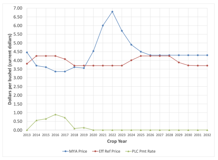
Figure 2. PLC payment rate factors for corn, 2013 – 2032
Notes: MYA prices for 2022-2032 are from USDA baseline estimates. The “Eff Ref Price” measures are the result of carrying out the steps in Table 1.
This effect of the maximum reference price can be seen more clearly in figure 2, where the plotted data only includes the MYA price, the effective reference price for PLC (i.e the outcome of applying the steps in table 1), and the PLC rate calculated as the difference between the PLC effective reference price and the MYA price (when that difference is greater than zero). Under the current reference price structure, the PLC program would have produced payments in years 2014 to 2019, though the current PLC effective price calculation (recall Table 1) only came into being with the 2018 Farm Bill[5] and was first used in the 2019 crop year.
The complex trigger mechanism of the PLC program has three distinct components. The moving average component is the type we might expect in an income support environment where steep falls in prices are met with support funds to help transition decision makers as the price environment changes rapidly. The lower boundary set by the reference price is an instrument of pure price protection that we might expect to be set based on its relation to the expected long run average cost of production[6]. Finally, the upper boundary in place that nullifies a “too high” moving average component is what defines the program as “shallow loss” support – indicating that the aim of the PLC program is to play a limited role, with excessive losses mitigated elsewhere in the farm safety net through crop insurance.
The lower and upper bounds created by the fixed reference price create a “band” of the minimum and maximum effective reference prices for calculating PLC payment rates. The data in Figures 1 and 2 indicate that the PLC program is limited in a dynamic price environment. This is particularly evident looking at the forecast price series that anticipates a long run equilibrium price above the upper bound of the effective reference price for corn. The inability of this band of effective prices to adjust to economic conditions limits the PLC program from performing its shallow loss function as the PLC rates drop to zero and remain there in an economy where output prices and input costs have surpassed the maximum effective price.
Examining PLC price triggers for other crops
The same plots for MYA price and PLC effective price components seen for corn in figures 1 and 2 are repeated in figures 3(a, b) and 4(a, b) for soybeans and wheat respectively. In figure 3a we see that the price and PLC component pattern for soybeans holds very similar to that of corn. Specifically, we see that PLC rates above zero are only seen prior to the 2019 crop year when the current PLC effective price rules were implemented under 2018’s Farm Bill. The increasing prices from 2020 to 2022 take prices to a level that raises the moving average component above the reference price ($8.40/bu for soybeans) from 2024 going forward. Indeed, the strong prices from 2020 to 2022 are high enough that the long run forecast MYA prices going forward to 2032 are all higher than the maximum reference price of $9.66/bu for soybeans.
Figure 3a. MYA and policy prices for soybeans, 2013 – 2032
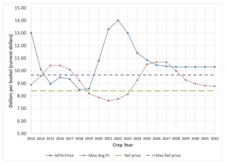
Figure 3a. MYA and policy prices for soybeans, 2013 – 2032
Notes: MYA prices for 2022-2032 are from USDA baseline estimates. Olympic average prices for 2022 forward use the projected MYA prices 2022-2032.
Figure 3b. PLC payment rate factors for soybeans, 2013 – 2032
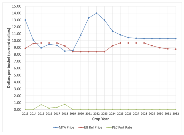
Figure 3b. PLC payment rate factors for soybeans, 2013 – 2032
Notes: MYA prices for 2022-2032 are from USDA baseline estimates. The “Eff Ref Price” measures are the result of carrying out the steps in Table 1.
The pattern for wheat MYA prices and PLC effective prices is like that of corn and soybeans but the level of MYA prices relative to reference prices is different. The peak prices from 2020 to 2022 are well above the maximum effective reference price but the long run MYA price forecast is firmly within the band of effective price factors ($5.50/bu to $6.33/bu). In figure 4b we see that PLC rates we calculate are above zero from 2014 to 2019 and during the projected price period from 2022 forward there are positive PLC rates 2026 to 2028.
Figure 4a. MYA and policy prices for wheat, 2013 – 2032
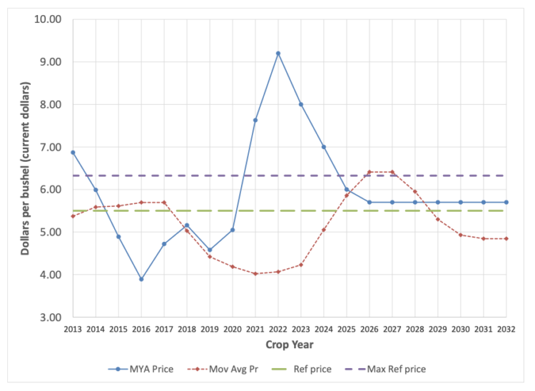
Figure 4a. MYA and policy prices for wheat, 2013 – 2032
Notes: MYA prices for 2022-2032 are from USDA baseline estimates. Olympic average prices for 2022 forward use the projected MYA prices 2022-2032
Figure 4b. PLC payment rate factors for wheat, 2013 – 2032
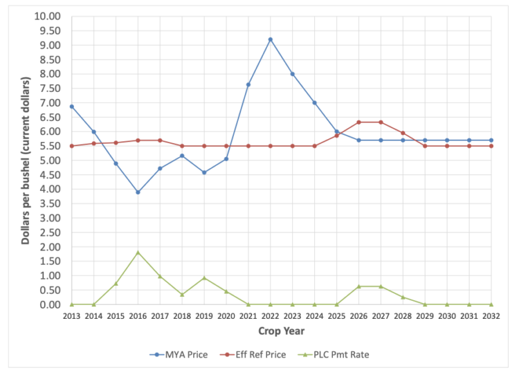
Figure 4b. PLC payment rate factors for wheat, 2013 – 2032
Notes: MYA prices for 2022-2032 are from USDA baseline estimates. The “Eff Ref Price” measures are the result of carrying out the steps in Table 1.
Returning to the previous consideration of the purpose of PLC and its effective reference price defining the program as shallow loss we see that the level of prices is key. Taken in isolation, the inability of the band of the PLC’s effective reference price would limit the program’s effectiveness. This is particularly true if we expect price patterns that are similar across crops to drive input costs to levels that shorten profit margins across the board. This integrated nature of crop prices with crop input costs is considered typical of competitive markets like we see in commodity agriculture.
While the combined historical and forecast price era we examine here is not typical as several economy-wide shocks have driven year over year price increases, the current price era does illustrate the limitation of the PLC program’s effective price calculation. Specifically, some mechanism to move the band of price protection in a way that reflects the reference price relative to input costs would more adequately reflect the shallow loss objective.
PLC and other components of the farm safety net
In the previous section we considered PLC “in isolation” but the farm safety net is much broader than the PLC program. As the farm bill commodity title has shifted from income and price support to risk management the role of crop insurance has greatly expanded. Crop insurance contracts are offered on an annual basis and will most accurately reflect current market conditions when coverage and rates on offer are published. If the purpose of the PLC is to provide shallow loss coverage to replace deductible losses, then the limitation of the fixed effective price band remains and indicates the PLC program is not particularly complementary to crop insurance.
However, PLC is not the only “shallow loss” option for producers in the commodity title. We have not discussed the Agricultural Risk Coverage (ARC) programs that producers can elect as an alternative (see footnote 1). The ARC program works as revenue protection and uses a similar moving average price component in the calculation. We do not go into the program’s formula here other than to note that a period of increased and sustained price increases (at trend yields) avoids the fixed band issue of PLC but still offers limited shallow loss protection if commodity price increases are twinned to per unit input costs. Of course, yields can be quite variable around their trend, marking ARC with different functionality vis-à-vis prices than PLC altogether.
Finally, both PLC and the ARC alternative are payments based on a historical allocation of base acres and not the actual crop production plan for a given year. The use of historical acreage introduces a measure of decoupling, severing any linkages between a farmer’s planting decisions and the level of commodity payments. The shallow loss objective will be retarded by any differences in historical base acres and current planting. This means for producers with a marked difference between historical base and current planting acreage we should view PLC (and ARC) as something of a basic income support program – an objective that would also by limited by the failure of program effective prices to reflect large changes in prices that pass through to increased input costs.
Concluding thoughts
The farm safety net has evolved in purpose from income support to risk management over the past twenty years and that has been reflected in the succession of farm legislation passed from 2002 and 2018. The priority of farm groups for the 2023 Farm Bill is sustaining the federal crop insurance program. The current PLC option of the commodity title is the product of its own sort of evolution, dating back to the 1996 Farm Bill when the primary mechanism for income support was changed to decoupled direct payments that paid fixed rates on fixed historical base acreage. Revisions to the commodity title over time has sought to re-couple payments to current market conditions while keeping them divorced from current managerial decisions. The effect has been to create a PLC program option that is difficult to classify in terms of an explicit policy objective within the farm safety net.
Successor legislation to the 2018 Farm Bill might address some limitations of the PLC program option made evident by the current commodity price era as outlined in this brief. Such modifications might take the form of additional steps in the calculation of an effective price (see table 1) or could be a directive to the Secretary of Agriculture to make adjustments to the fixed reference price under qualifying conditions. Whatever form that revision might take, it will be important to consider the objective of the PLC program option in the broader safety net context and whether that may require more than just adjustments to the PLC effective price structure. If the PLC program is to continue as a shallow loss adjustment, then the PLC program definitions must incorporate the notion of loss beyond changes in price relative to some fixed reference point.
[1] The alternative to the PLC program uses prices and yields to build a revenue based trigger.
[2] An olympic average price is calculated by dropping the highest and lowest value of the set and then averaging the remaining values.
[3] This has the effect of adding an extra year of “lag” between the calculated olympic average price and the year it is calculated. For example, the 2022 olympic average price in reference price calculations would use 2016 to 2020 MYA prices in the calculation because at the start of the 2022 crop year the 2021 MYA price is not known.
[4] The PLC program began with the 2014 crop in that year’s farm bill and was adjusted to the current set of price triggers in the 2018 farm bill. We apply it backwards (and forwards over projected prices) here to illustrate the program mechanisms.
[5] The PLC program from the 2014 Farm Bill (2014 to 2018 crop years) did not feature a moving average component to increase the effective reference price above the fixed statutory price. This means the PLC rates shown here are overstated relative to the program rules in effect at that time. Because our purpose here is to examine the economic mechanisms of current law we maintain the 2018 Farm Bill effective price rules consistently over the historical and projected price series used.
[6] The Farm Bill incorporates a “loan rate” setting a price floor under crops as a pure measure of price protection. The loan rates are for crops are set below the statutory reference prices of the PLC program.
![]()
![]()
![]()
![]()
![]()