Indiana Farmland vs. Alternative Investments

Farmland is the primary asset of agricultural production. According to the USDA, the U.S. has roughly $2.6 trillion of farm real estate, which accounts for approximately 83% of the value of total farm sector assets (USDA ERS). As a result, farmland is typically the largest single investment and the primary store of farm sector wealth. In addition, farmland’s historic performance for stable and predictable returns make it an attractive asset class for investors beyond farm operators. Given the significant financial commitment required for farmland ownership, it is important to understand how farmland, as an asset class, compares to other investment options. Our analysis shows that farmland offers relative stable set of returns across most investment horizons. Farmland offers total returns that approach those of equities but with substantially lower risk.

Table 1, below, provides a summary of several major investment options over four investment horizons: 1980 – 2020, 1990 – 2020, 2000 – 2020, and 2010 – 2020. Investments are evaluated according to three common measures. First, the mean represents the expected return over the investment horizon, in percentage points. For example, Table 1 shows that the Dow Jones Industrial Average had a mean return of 9.8% between 1980 and 2020 and a mean return of 11.0% in the recent decade from 2010 to 2020. Second, the standard deviation (St.D.) represents the variation in returns over the investment horizon. The standard deviation therefore measures the variability or riskiness of the investment. Again, the Down Jones Industrial Average had a standard deviation of returns of 15.6% between 1980 and 2020 and 8.3% from 2010 to 2020. Third, the coefficient of variation (CV) is a ratio calculated as the standard deviation divided by the mean return (St.D./Mean). Thus, the coefficient of variation represents the relationship between expected return and riskiness of an investment. Economic theory suggests that risk averse investors are only willing to take on additional risk if they are compensated by a higher expected return. As a result, risk averse investors prefer investments with lower coefficient of variation. For example, between 1980 and 2010 the Dow Jones Industrial Average exhibited a coefficient of variation of 1.6, but over the same period, AAA corporate bonds had a coefficient of variation of 0.4. While the Dow Jones Industrial Average had a much higher mean return (9.8% vs. 7.2), the returns were substantially riskier (15.6 vs. 3.0). Thus, a highly risk averse investor would prefer to hold AAA corporate bonds over the equities represented by the Dow Jones Industrial Average.

The investments summarized include a mix of equities, bonds, and other asset classes. The equities include two common stock indices: the Dow Jones Industrial Average (DJIA) and the Standard & Poor’s 500 (S&P500) indices. For each index, the returns are calculated as the percentage change in index value from the last trading day of June in one year to the last trading day of June in the previous year ( ). The next two investments are bond yields (in percentage points): ten year U.S. treasury bond (Treasury (10)) and AAA-rated corporate bonds (AAA). The bond yields are similarly based on end of June trading values. The final two investments include the Federal Housing Finance Agency all-transactions U.S. residential housing price index (Housing) and gold prices based on the London Bullion Market Association 3:00PM fixing price (Gold). The final row of Table 1 includes the Consumer Price Index (CPI) inflation measure. As a general rule, investors prefer assets with expected returns that exceed the rate of inflation in order to preserve the nominal value of an investment over time.

Table 1 shows that equities offer the greatest mean return across all investment horizons. However, equity investments also exhibit higher standard deviation of returns. As a result, the risk averse investors would prefer a portfolio with larger allocations to bonds which offer lower but more stable returns, as represented by the coefficient of variation.

Table 1: Expected returns and risk of alternative investments

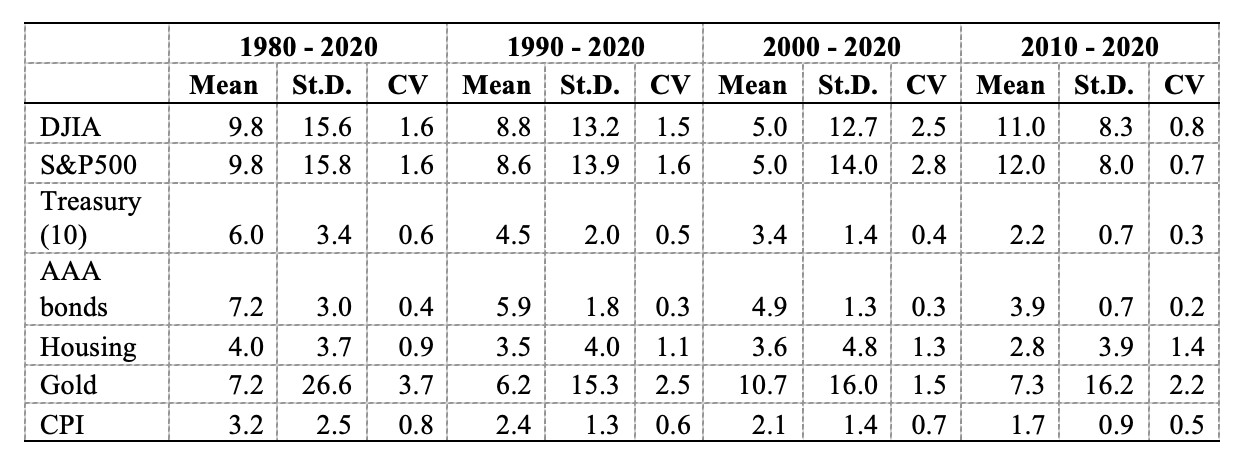
Table 1: Expected returns and risk of alternative investments

Table 2 similarly reports the returns to Indiana farmland as captured by percentage change in values obtained from the Purdue Land Values and Cash Rents Survey. Across all potential investment horizons, Indiana farmland values appreciated at a rate below the mean returns to the equity indices but above the returns of government or corporate bond yields. For most horizons, Indiana farmland price appreciation rates were less volatile than the returns to equities yet were substantially riskier than bonds. Farmland owners were compensated by the riskiness of their investment relative to other asset classes, as measured by the coefficient of variation, however, excluding the period that includes the 1980s Farm Financial Crisis.

Table 2: Expected returns and risk of farmland as measured by price appreciation

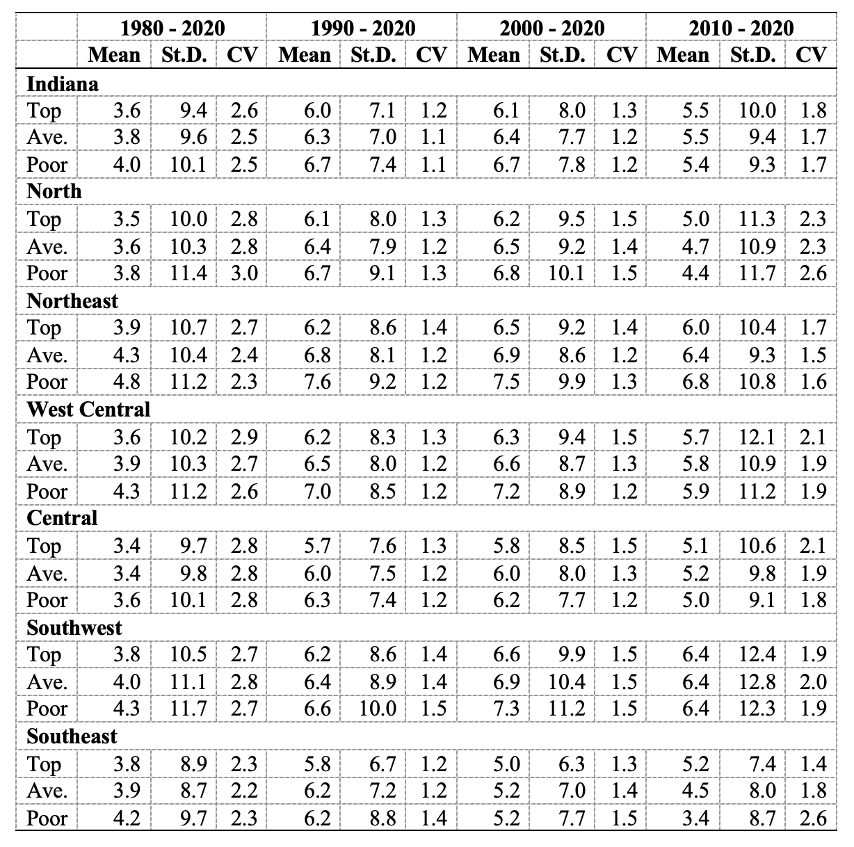
Table 2: Expected returns and risk of farmland as measured by price appreciation

Farmland price appreciation, however, is only one source of returns that accrue to farmland owners. In addition to price appreciation, farmland ownership includes the returns to agricultural production. Table 3 similarly reports the three measures of the risk and return to farmland ownership that includes both appreciation and the income component, as measured by average cash rental rates. When the income component is included in the measure of return, farmland offers a substantially higher expected return with a marginal increase in riskiness (as measured by standard deviation of returns). As a result, when one considers the total returns to farmland ownership, the asset represents a more attractive alternative to equities and bonds.

A third source of return is the potential to convert farmland to other land use types, such as residential or commercial uses. However, for the purposes of this research, we limit our analysis to farmland that is held in agricultural production in perpetuity. Previous Purdue Land Value and Cash Rent Surveys suggest that farmland sold for development is typically associated with a sales price that is approximately twice that of top quality farmland.

Table 3: Expected returns and risk of farmland as measured by price appreciation and cash rents

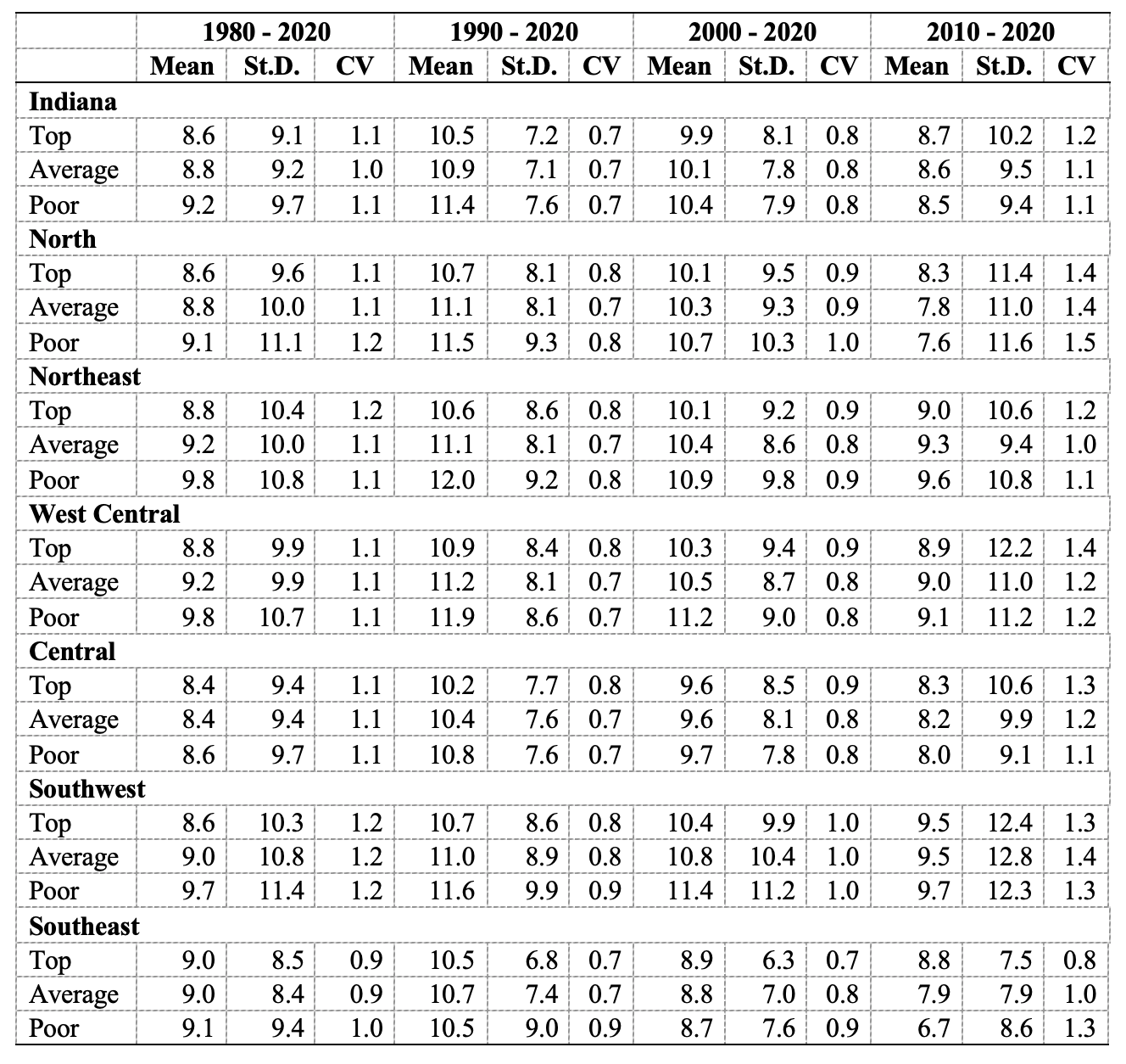
Table 3: Expected returns and risk of farmland as measured by price appreciation and cash rents

Farmland, as an asset class, is also lauded given its relationship to other investments in a diversified portfolio. A portfolio is well diversified if the returns of each investment are independent of the returns to other investments, or, in other words, if the correlation in investment returns is low. Alternatively, some asset classes can be a valuable addition to a well-diversified portfolio if the returns are inversely correlated with those of other investments. That is, the returns tend to move in opposite directions as the other investments, or as the returns to one asset increase, the returns to the others tend to decrease. Table 4 shows the correlation between farmland price appreciation and the other investments considered in Table 1. Table 4 suggests that farmland has low levels of correlation with many investment options, including equity indices and gold. In addition, farmland is inversely correlated with bond yields and housing. Thus, as bond yields fall, farmland prices tend to rise.

Table 4: Correlations between returns to farmland and other investment alternatives

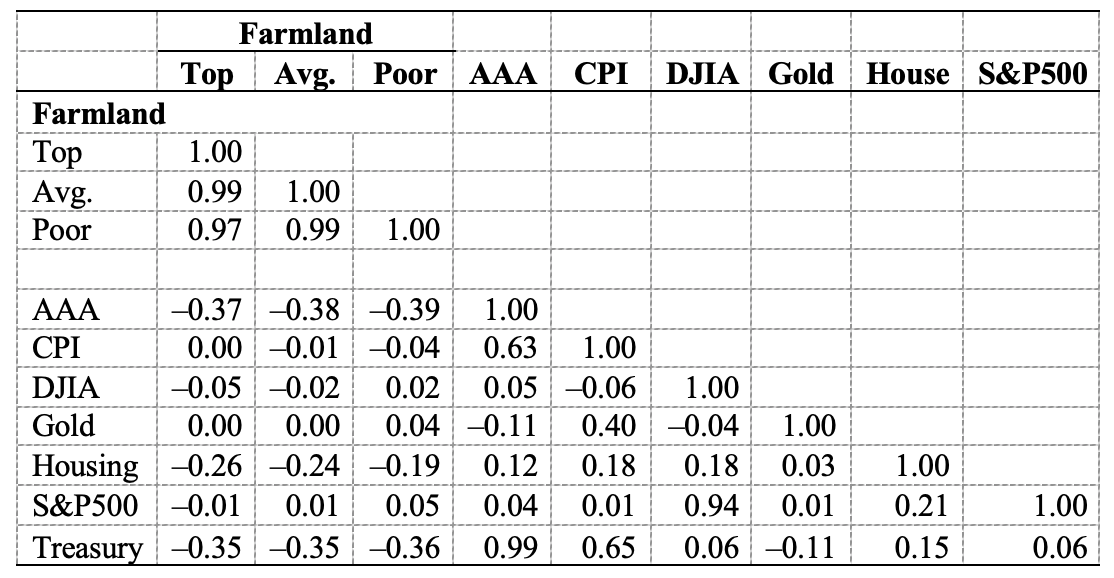
Table 4: Correlations between returns to farmland and other investment alternatives