July 18, 2012
When Do Farm Booms Become Bubbles? (Manuscript)
![]()
![]()
![]()
![]()
![]()
Introduction
Rapid increases in agricultural incomes and asset values have brought back memories of previous booms and busts. Henderson, Gloy, and Boehlje (2011) chronicled previous agricultural booms and busts noting that they have often corresponded to rapid expansions and contractions of agricultural exports. As in previous eras, today’s agricultural boom has been fueled by increases in export demand. A key difference however, is the dramatic increase in domestic demand associated with the use of biofuels.
Throughout agricultural history, dramatic increases in income have generated substantial supply responses as farmers around the world invested to meet increased demand. If demand expansion proved to be transitory, the supply response brought with it a corresponding price correction that substantially reduced agricultural commodity prices and incomes.
Agricultural production is a relatively capital-intensive business, requiring substantial investment in equipment and farmland. Fluctuations in agricultural incomes present farmers, and almost all businesses associated with the agricultural sector, significant capital allocation challenges. The capital investments made today will generate returns for many, many years into the future. Determining the appropriate price to pay for capital assets and the appropriate amount of investment in capital equipment is critically dependent upon how investors view future economic conditions. The fluctuating nature of agricultural prices makes forecasting these conditions challenging.
Because agriculture is capital intensive, positive income shocks generate significant returns to fixed assets that were purchased based upon expectations of more modest incomes. These newfound windfalls present firms with a dilemma. If the demand shock persists, the existing capital stock is likely substantially undervalued, and there is tremendous pressure for the value of these assets to increase. If the shock proves temporary, supply quickly catches up with demand, incomes fall, and assets purchased on the expectations of higher incomes become overvalued.
The magnitude of recent demand increases have occurred relatively infrequently throughout modern agricultural history. Instead, most in agriculture are more familiar with weather-induced supply shocks, which tend to be short-term in nature. These shocks are frequently recognized as times of high prices that will only last until growing conditions return to more “normal” times. In this situation, asset prices do not typically undergo substantial upward price movement. Indeed, the picture over most of agricultural history is one of generally declining real commodity prices as productivity gains offset marginal demand increases. When demand appears to undergo a substantial outward shift, it calls into question whether the long-term trend toward declining real commodity prices remains in place, setting the stage for rapid appreciation of agricultural fixed assets, namely farmland.
While recent demand shocks alone are likely sufficient to substantially increase asset values, they have occurred during a period of historically low interest rates. Interest rates are an important component of the story with respect to farmland values and capital allocation, because they influence the rate at which future earnings are discounted to today’s dollars. Higher interest rates reduce the value of future earnings and lower rates increase their value. Today, rates are clearly low, so at the same time that agricultural incomes have increased, rates have declined, setting the stage for very rapid increases in agricultural land values (Gloy, et al., 2011).
As the rapid run up in agricultural incomes has been capitalized into farmland values, it has called into question whether the farmland market is responding rationally to the situation. In other words, do farmland prices reflect their underlying economic fundamentals or are they in a bubble? While farmland prices have increased across the United States, the most dramatic increases have been concentrated in the corn-belt region. For example, according to Iowa State’s annual farmland survey, average farmland values have increased 248 percent from 2001 to 2011, for an annualized growth rate of 13.3 percent, and average quality Indiana farmland has increased from $2,264 per acre in 2001 to $5,468 per acre in 2011 (Duffy, 2012; Dobbins and Cook, 2011).
The United States has experienced several dramatic price escalations and collapses across a variety of markets from technology stocks to housing, and the obvious question has arisen as to whether the farmland market is also now a bubble that will eventually collapse. This paper seeks to provide some insight on this issue. It first describes the concept of a bubble from the perspective of economists. It is pointed out that using the classic economic definition of a bubble, asset bubbles are extremely rare events and that trying to identify them with foresight is unlikely a worthwhile venture.
On the other hand, despite not meeting economists’ definition of a bubble, dramatic price inflations and collapses are certainly interesting, worthy of examination, and capture the attention of investors and the public. Realizing this, economists have found that the connection between investor expectations and economic fundamentals play a key role in these situations. The paper examines the farmland market fundamentals and reports on the findings of a survey of farmland investors with the goal of understanding the relationship between current farmland values and expectations.
Using economists’ definition of a bubble, it is unlikely the farmland market is currently in a speculative bubble. However, the analysis in this paper indicates that there are some reasons to be concerned about whether the current level of increases in farmland values are likely to be sustainable. Fundamental trends appear to be slowing, and there is some evidence that investor expectations may be only loosely tied to economic fundamentals, but the results are hardly conclusive. In the end, the outcome will depend upon the realization of a number of uncertain events surrounding demand and supply responses.
What is a Bubble?
There have been numerous examples of assets that have seen spectacular price increases only to be followed by collapses. Frequently these occurrences are labeled as asset price bubbles. Economists have studied many of these episodes in order to better understand why asset values behave in this manner. In doing so, most economists define bubbles as situations where asset prices increase at a rate that is not justified by the future income they are expected to generate. For instance, Malkiel (2012) defines a bubble as a:
“substantial and long-lasting divergence of asset prices from valuations that would be determined from the rational expectation of the present value of cash flows from the asset” (page 3).
Stiglitz (1990) offers another definition:
“If the reason that the price is high today is only because investors believe that the selling price will be high tomorrow –when “fundamental” factors do not seem to justify such a price –then a bubble exists” (page 13).
These definitions of a bubble are relatively clear. Investors should value an asset based upon their expectations of the value of the earnings that it will produce in the future. While the definitions are clear, determining how to test for a bubble using them is not particularly obvious. In order to identify a bubble,one must understand if its price is tied to investors’ expectations of future fundamentals. While current prices are easily observable, investor expectations are not, and testing has presented a challenge to many skilled researchers.
Using a definition that relies upon determining whether asset prices could have possibly been explained by some view of fundamental conditions, it has been pointed out that many frequently cited examples of asset bubbles could be plausibly explained by the conditions of the time. For example Garber (1990) carefully examines some of the most famous asset price inflation and collapses including the tulip mania, Mississippi, and South Sea bubbles and illustrates how each had reasonable economic interpretations that would disqualify them as speculative bubbles. Siegel even illustrates that if one examines a long enough time period, it is possible to conclude the dramatic stock market crashes in 1929 and 1987 did not meet economists’ definition of a speculative bubble. Similarly, Malkiel (2003) also describes several of the apparent violations of the efficient market hypothesis and argues that the model is well supported by almost all available evidence.
As Malkiel (2012) notes, even with the benefit of hindsight, it can be very difficult to detect a bubble. This makes detecting them ex ante very difficult if not impossible. It is unlikely that the farmland market is any different from these previous examples. This means that it is highly unlikely that the farmland market is in a situation that would conform to the standard economist definition of a bubble.
Unfortunately, this does not provide much comfort for those concerned with whether the potential might exist for farmland values to decline as spectacularly as they have risen. As Barlevy points out, the press and general public usually use the term “bubble” to describe the situation where prices increase and decrease significantly in a short period of time. Perhaps, many of these episodes did not satisfy the traditional economic definition of a bubble, but clearly,it is worth studying the dynamics that lead to such spectacular price increases and collapses.
Whether called bubbles or not, these spectacular price increases are often driven by exogenous factors that can be rationally interpreted as greatly increasing expectations of future profits that an asset will generate (Malkiel,2012). These changes alter investor expectations and create uncertainty. Shiller points out that the economist view of asset prices (and bubbles) depends critically on investor expectations (1990; 2003). Although,one observes the outcome of expectations (prices), one rarely observes the actual expectations that drive these prices. In studies where he surveyed individuals in different real estate markets, he notes that investors exhibited little apparent interest in quantitative evidence about fundamentals, instead simply attributing price movements to whatever seemed to be the most plausible fundamental explanation.
Further, Shiller describes how feedback loops between prices can play a role in developing further price increases and decreases (2003). Basically, he argues that high prices can encourage higher prices (and vice versa). Such a loop is not consistent with fundamentals determining asset prices. His findings illustrated the importance of understanding the models that investors used to derive asset values. In his 2011 interview with the Financial Crisis Inquiry Commission, Warren Buffett offered a similar explanation of bubbles in which he focuses on the price feedback mechanism:
“The only way you get a bubble is when basically a very high percentage of the population buys into some originally sound premise –and it’s quite interesting how that develops –originally sound premise that becomes distorted as time passes and people forget the original sound premise and start focusing solely on the price action.” (page 3)
The current situation in the farmland market certainly exhibits some of the features that are described by Malkiel, Shiller and Buffett. The current price increases have been driven by changed fundamentals outlined in the introduction, increased demand, reduced interest rates and negative short-term supply shocks. While the negative short-term supply shock can likely be ruled out as a cause for a long-term upward re-valuation of farmland, the emergence of a new and growing source of demand could plausibly justify upward re-valuation of farmland prices. A central question is then whether the market participants are still focused on evaluating these fundamentals or whether other factors are driving prices higher.
Many readers will not be comforted by the claim that it is highly unlikely that the current situation in the farmland market fits the classic economic definition of a speculative bubble. These situations rarely, if ever, occur. Given previous experience with rapid farmland price appreciation in the 1970s and declines in the 1980s,it is certainly possible that farmland prices can descend as quickly as they increase. Since nearly 85percentof the farm sector’s wealth is tied to the value of farmland, it is certainly important to understand farmland price movements. The next section describes some of the most important fundamental factors and their trends. Then, the question of how market participants perceive values and fundamentals is addressed.
Farmland Values and Fundamentals
Farmland markets in most of the U.S. corn-belt have experienced substantial price appreciation since roughly 2001. For example, average quality Indiana farmland has appreciated by 145percentover this time period (Dobbins and Cook). The increases in Iowa have been even more dramatic, with the statewide average increasing from $1,926 to $6,708 per acre,or 248percent,from 2001 to 2011 (Duffy). For thefirst time since they began their survey in the 1970s, the Kansas City Federal Reserve Bank reported that farmland values in their district rose by more than 20 percent for two consecutive years (Henderson and Akers, 2012).
A Historical Perspective on Nominal and Real Gains
In nominal terms the relative increases in farmland values today are not as large as those experienced in the 1970s (Table 1). For example, over the 10-year period of 1971-1981,average Iowa farmland prices rose nearly 400percent, andU.S. farmland values rose 300percent. However, it is important to remember that the 1970s was a period marked by relatively high rates of inflation. When converted to real values, the rates of increase experienced in the last 10 years are actually much closer, and in the case of Iowa, exceed those experienced in the 1970s (Table 1). In the case of Illinois,the real changes for these periods are remarkably similar. In contrast, the 1970s were a period of more rapid real and nominal growth in Indiana and the United States in total.
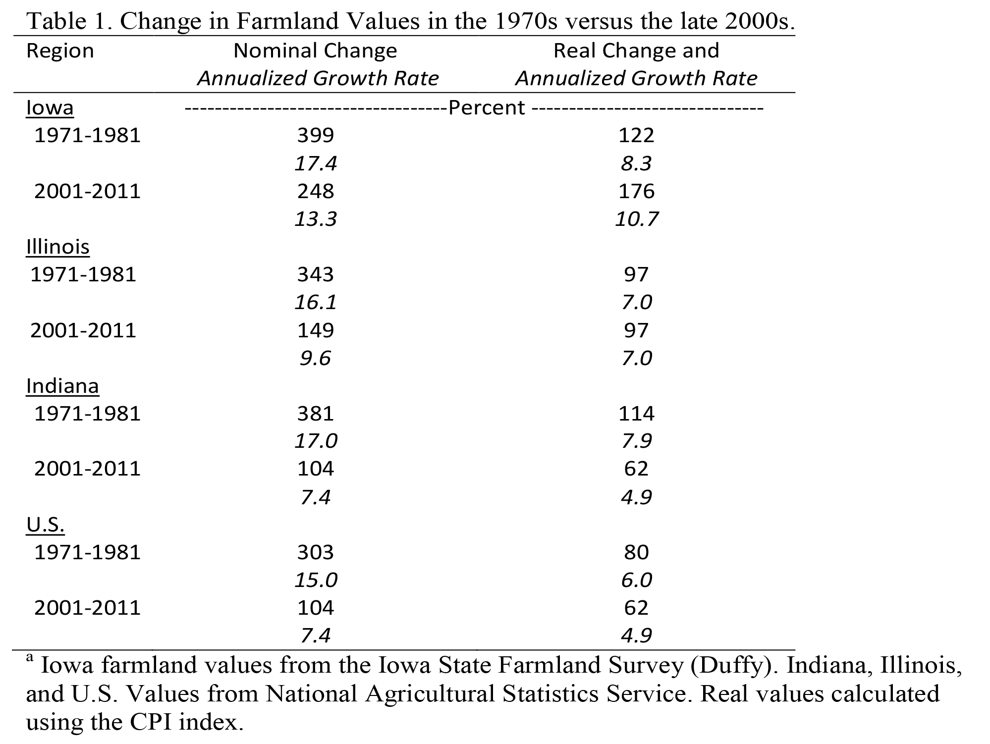
Table 1. Change in Farmland Values in the 1970s versus the late 2000s.
The above table illustrates that the increases occurring today are on par with those that occurred in the 1970s. Table 2 illustrates how farmland has appreciated in Iowa over a wider range of time periods. This table shows the annualized change in the real value of Iowa farmland over selected periods from 1961 to 2011. For the five time periods shown since 1961, Iowa farmland values have increased at an annual rate between 0 and 5 percent, with the 20-year period from 1961 to 1981 being particularly good, and the 30-year period from 1961 to 1991 showing next to no appreciation. The time from 1981, the peak of the last rapid period of farmland increases, to 1991 is the worst of the periods shown, when farmland decreased in real value at annual rate of 9percent. The best of the periods shown is the most recent, where real farmland values increased by 11percentper year.

Table 2. Annualized Real Rate of Change in the Value of Iowa Farmland, Various Periods, 1961-2011.
Increasing Value-to-Rent Multiples
The previous results further reinforce how strong the recent real gains in farmland prices have been. These dramatic increases have occurred as both the income produced by farmland and the amount that investors are willing to pay for that income has increased. The value-to-rent multiple is a commonly used metric of farmland valuation. This ratio of the price of land to its current cash rental rate provides a measure of how expensive land is relative to the current income that it generates. Currently, the value-to-rent multiple is near all-time highs for most areas of the corn-belt (Figure 1). For example, according to the USDA, average quality cropland in Iowa now sells for roughly 29 times its cash rental rate. Similar multiples hold for Indiana and Illinois. In other words, buyers are willing to pay roughly $30 for each dollar of current gross cash rental income.
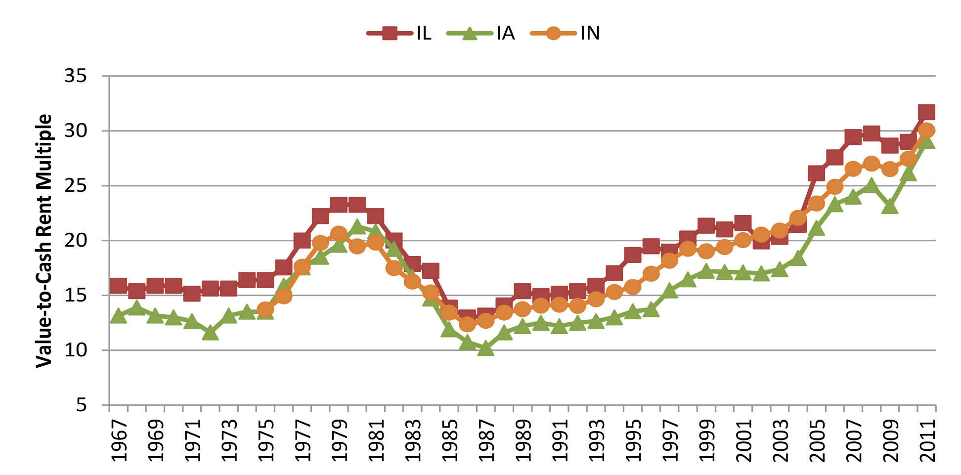
Figure 1. Value-to-Cash Rent Multiple for Illinois, Iowa, and Indiana Cropland, 1967-2011.
Sources: Iowa and Illinois data were compiled from various Land Values and Cash Rent Summary reports published by the National Agricultural Statistics Service. The Indiana data are from the Purdue Annual Land Value Survey, June 2011.
Judging from the graphic, this rate is high by most historical standards. Before the early to mid-2000s,the previous peak in the value-to-rent multiple occurred in the late 1970s and early 1980s when it topped out between 20 and 25 depending upon the specific state.
The current magnitude of the value-to-rent multiple is one signal that prices for farmland are high relative to earnings. However, this multiple must be interpreted with some caution as it relates only current income to farmland prices. Farmland will generate earnings for many periods into the future and a high multiple could very well represent the fact that most investors expect that income will rise rapidly in the future. Likewise, the magnitude of the multiple is influenced by rates of return on competing investments. Because interest rates are low, investors are generally willing to pay more for future earnings, thus pushing the multiple higher.
A Historical Perspective on Sector Returns and Asset Values
In the period leading up to the last farm crisis, Melichar(1979) conducted a thorough analysis of farmland returns and illustrated how growth expectations could generate farmland value-to-rent multiples of 30. His analysis showed that real returns to productive assets in agriculture grew substantially before and during the 1970s. If farmland is capable of persistently producing real growth rates in the range of 3 percent to 4 percent, it would not be unrealistic to expect that farmland could trade at a multiple in the 30s. However, it is also likely that persistent real income growth of that magnitude or very low interest rates would be necessary to maintain such a multiple over a long period of time.
There are a variety of income measures that could be compared to asset valuations. Melichar (1979) argued that a simple comparison of net income to asset values in agriculture can be extremely misleading. Instead, he advocated that one should compare the returns to productive assets to their valuations. Figure 2 shows the net returns to farm operators plus rent paid to non-operator landlords and interest payments, which is a measure of the return to productive assets, unpaid labor and management. Interest expense and rents are added back because they are a component of the returns to debt and land owned by non-operators.
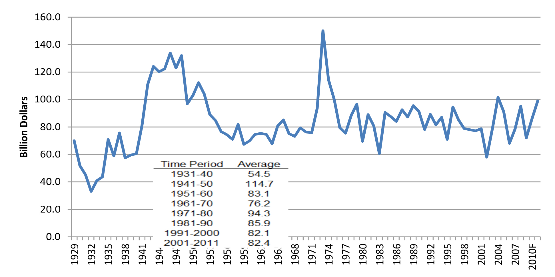
Figure 2. Return to Farm Operators plus Interest and Rents Paid to Non-Operator Landowners, 1929 –2011 (2005 USD). GDP chain type price index used to convert to real values.
The calculation differs from that found in Melichar(1979) because no charges were subtracted for unpaid operator labor and management. Thus, the series in Figure 2 would best be described as the net return to productive assets and unpaid labor and management.1 The values were then converted to 2005 dollars using a GDP chain type price index (ERS-USDA, 2012).
The chart shows the return to operators plus interest and rent since 1929 in constant 2005 dollars. Over this time period, the series averaged $83.6 billion and has frequently (74 percent of the time) fallen in a range from $60 billion to $100 billion. The large income shock associated with 1973-1975 is easily observed from the graph, but the most notable period of persistently high returns was associated with World War II. Only in the 1940s and early 1950s did returns consistently top $100 billion.
Recently, incomes have flirted with the $100 billion mark, topping it in 2004, approaching it in 2008, and forecast to touch it in 2011. It is also worthwhile to note that since 2000, returns have also been as low as $58 billion (2002), $68 billion (2006), and $71.9 billion (2009). While it is clear that,on balance,recent years have been very good in terms of the returns to productive assets, they are clearly not unprecedented in magnitude. A more thorough and detailed discussion of the causes of these historic income fluctuations can be found in Henderson, Gloy, and Boehlje (2011).
The return to operators plus interest and rent was then divided by the value of farm production assets, all in constant 2005 dollars. Production assets included real estate, inventories, and equipment. This ratio represents the rate of return to production assets and unpaid labor and management in the farm sector. Because the returns to management and unpaid labor are included in the numerator, the actual return to production assets would be lower than that depicted. Further, the rate of return is a return to all production assets, not just farmland.
Figure 3 shows the annual rate of return as well as its 5-and 10-year rolling averages. Over the entire period, the average rate of return to unpaid labor, management, and productive farm assets is 6.49percent. The rate of return can be quite variable, with a clear peak experienced in the early 1970s and a bottom of 3.41percentin 1980 when asset values had risen faster than incomes. When incomes dropped in the 1980s, production asset values, dominated by real estate, began to adjust downward to lift the rate of return back above 6percentby 1984.
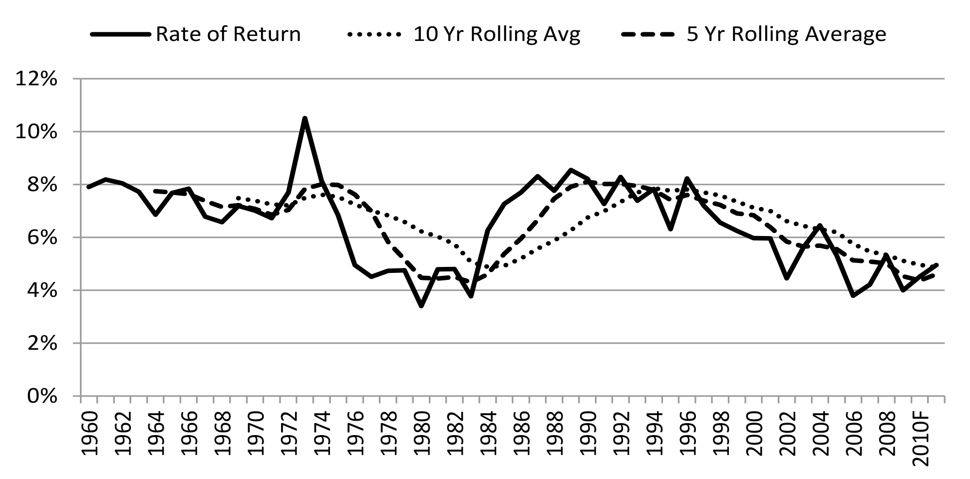
Figure 3. Returns to Farm Operators plus Interest and Rent Divided by Farm Production Assets, 1960-2011 (2005 USD).
Since roughly 1996, the rate of return has trended downward and is currently slightly less than 5percent. This chart further reinforces the findings associated with Tables 1 and 2,which illustrated that in real terms the increases in the value of farmland have been on par with those experienced in the 1970s. Given that incomes have been somewhat higher in the 2000s than the 1990s, the decline in the rate of return would indicate that asset values have increased relatively more quickly than incomes. In fact, even with the large positive income shocks in 2008 and 2011, the rate of return failed to exceed 6percent, last exceeding that level in 2004.
This figure would suggest that over the last decade investors have been willing to accept relatively lower rates of returns than in most previous time periods2. Overall, the falling rate of return on productive assets is related to the increasing value-to-rent multiples observed in the farmland market. It would appear that investors are content with lower rates of return or that they expect income to increase in the future.
Falling Interest Rates
It is plausible that some of the willingness to accept a lower rate of return on farm production assets is related to a general trend toward lower interest rates (Figure 4). Interest rates have declined substantially in the last 20 years. Falling interest rates have lowered the opportunity cost of alternative investments and have helped to support higher multiples (lower rates of return on productive assets). A decline in interest rates can have a substantial impact on multiples and valuations (Gloy, et al., 2011a, 2011b). For instance, the multiple associated with a 5 percent capitalization rate is 20,while it is 25 for a 4 percent capitalization rate. Growth expectations also should increase the multiple by decreasing the capitalization rate.
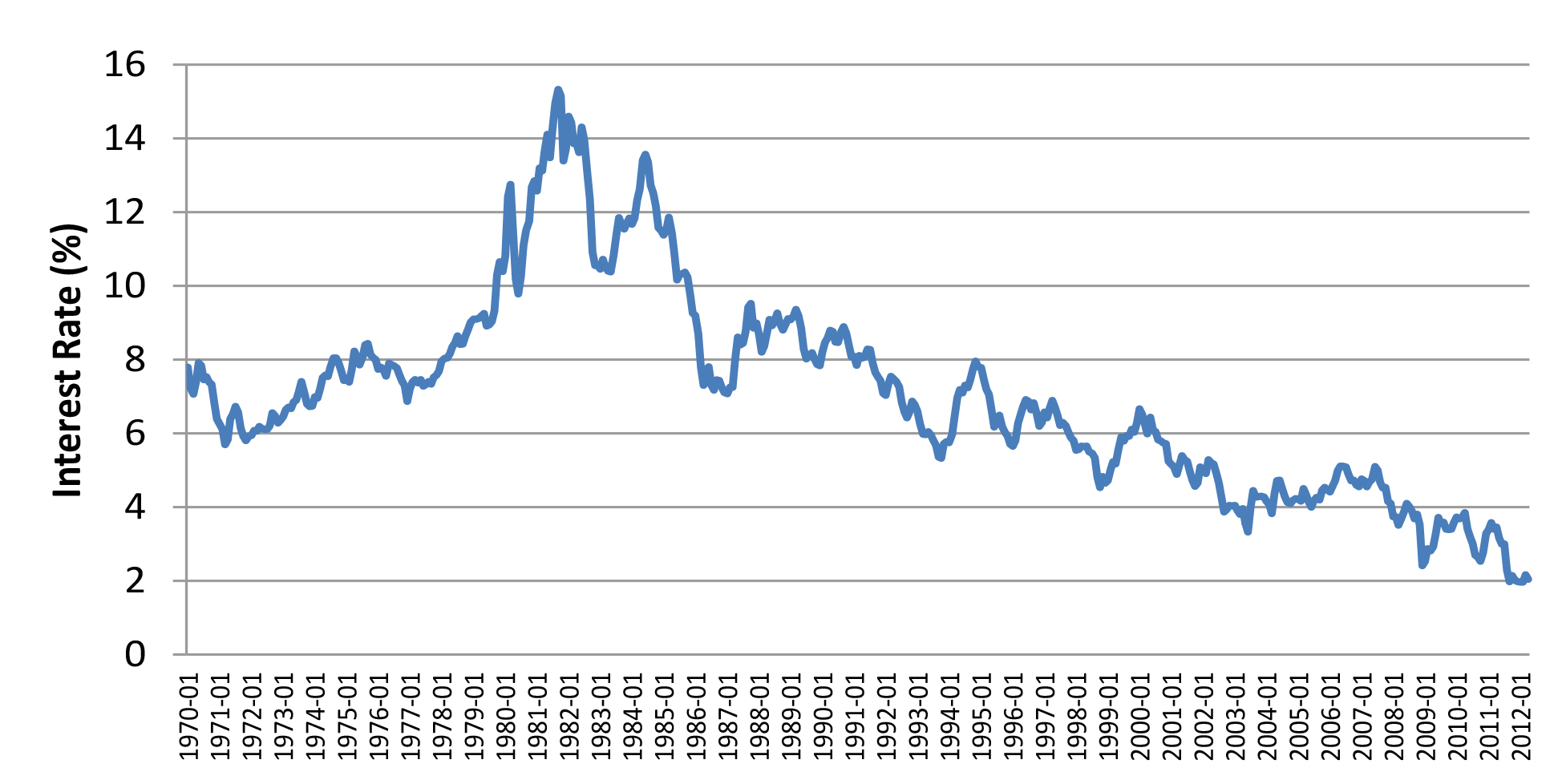
Figure 4. Monthly Average Interest Rate on 10 Year U.S. Treasury Bonds, 1970 –2012.
In general, increases in incomes and reductions in interest rates have led to increased farmland values. In real terms these values have increased substantially, on par with the magnitude of the increases observed in the late 1970s. It is clear that in order to justify these prices on the basis of economic fundamentals investors must have relatively optimistic expectations about future incomes and interest rates in order to support the current multiples. In other words, they must expect that incomes will rise and interest rates will remain low. It could easily be the case that such a situation will materialize.
Returns and Values: The Case of Indiana
While the previous discussion has been at the abstract level of sector wide returns and the value of production assets in the sector, most of the substantial increases in farmland values and incomes have been associated with row-crop operations. Figure 5 shows the budgeted profit (loss) and cash rental rates for high quality Indiana farmland from 1991 to 2012. The expected profits from farming have been very strong in recent years, in some cases exceeding the cash rental rate. This contrasts with the period prior to 2007,when expected profits were frequently negative. Although rents have increased since 2007, it is likely that they will continue trending upward if expected profits remain strong. If land values remain constant, such increases would work to reduce the value-to-rent multiple. However, to bring the multiples down,rents would have to increase at a faster rate than values.
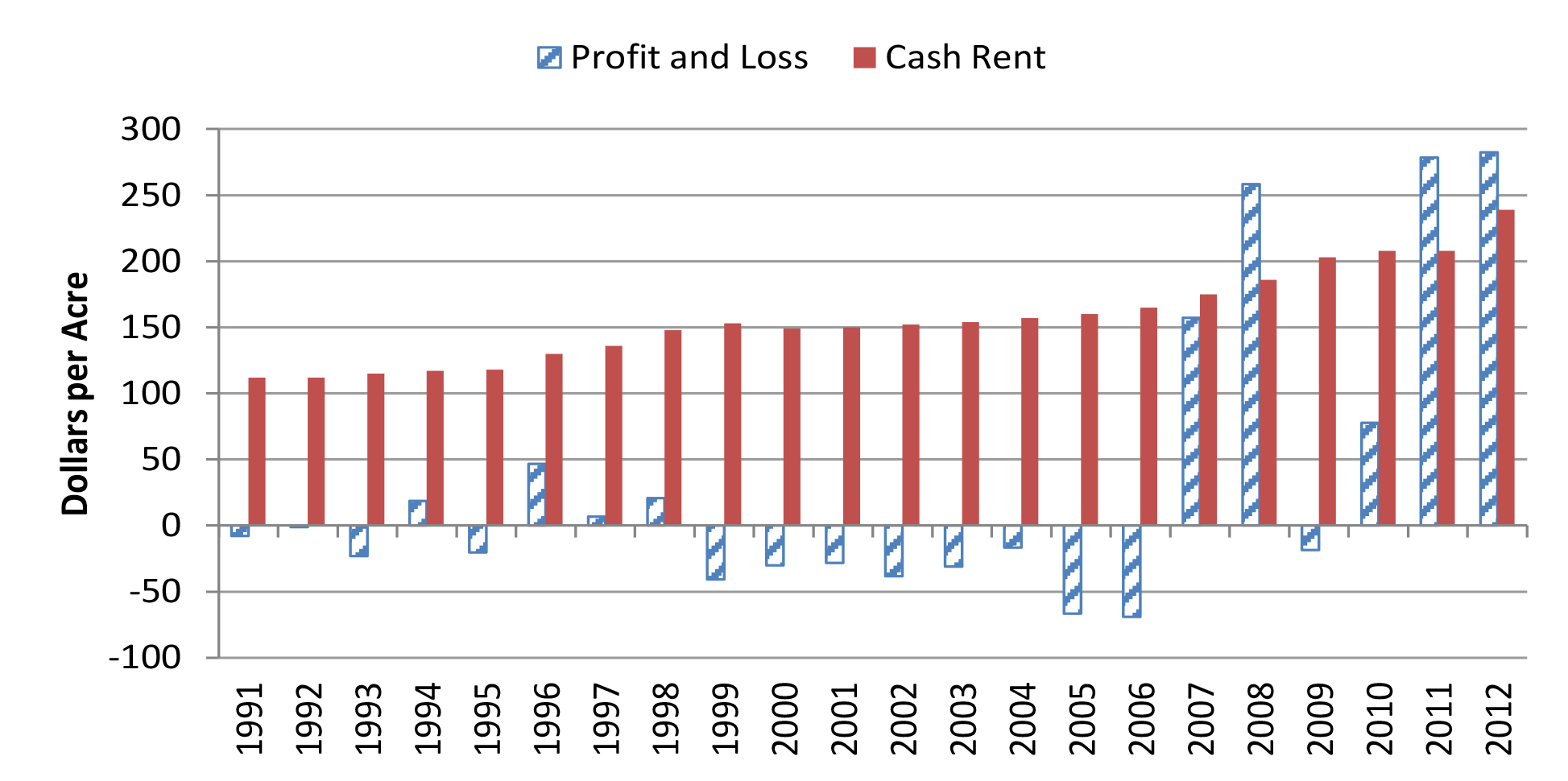
Figure 5. Budgeted Profit (Loss) and Cash Rental Rate, High Quality Indiana Farmland, 1991-2012.
Source: Derived from Purdue Crop Budgets, ID-166.
Finally, one can use the standard income capitalization model to examine how alternative capitalization and income expectations would influence farmland values.Gloy,et al. (2011a), describe such an analysis and some of its caveats in more detail. Figure 6 summarizes how different assumptions about the capitalization rate and income influence potential farmland values using the case of high-quality Indiana farmland.
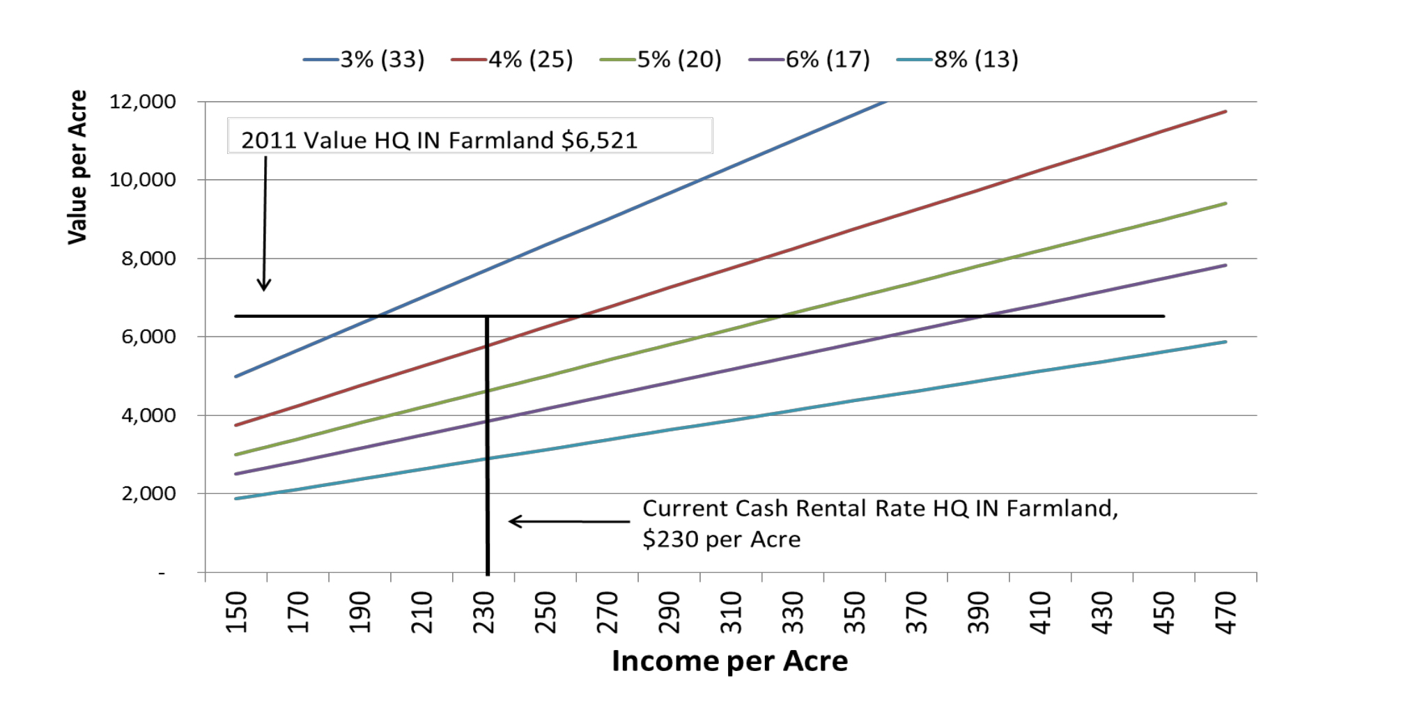
Figure 6. Land Values with Alternative Capitalization Rates (Multiples) and Income Levels.
The current value and cash rental income place the capitalization rate between 3 percent and 4 percent. Using this simple model, one could also arrive at such a price with a higher capitalization rate (lower multiple) if incomes were to rise. For example, if the capitalization rate were to rise to 5 percent (the multiple falls to 20), income would have to rise to roughly $330 per acre to maintain farmland values at $6,521 per acre.
Figure 6 illustrates the very large impact of low capitalization rates on farmland values. With frequent anecdotal evidence of farmland sales in excess of $10,000 per acre, it is reasonable to ask what capitalization rate/income combinations would give rise to such a price. One can see that at capitalization rates of 3 percent, such a price would require perpetual income of roughly $300 per acre. If the capitalization rate rose to a more historically common level of 5 percent (20 multiple), the expected perpetual income would have to rise to more than $500per acre to achieve a $10,000 per acre price. This would require much more aggressive assumptions about the future profitability of crop farming. What is obvious from these charts is that lower capitalization rates (higher multiples) greatly expand the likely range within which farmland values will trade.
Are the High Multiples Sustainable?
While the previous discussion provides some rationale for the idea that value-to-rent ratios could be maintained at current high levels, it is also worth noting that several factors could work against this.First, the high valuations are dependent upon growing income streams and/or low interest rates. If supply/demand conditions were to deteriorate, it is unlikely that rents would continue to grow. Without income growth, multiples of this level would be very difficult to support. Second, interest rates are relatively low. In order to maintain values at current levels, higher interest rates would require either that income growth accelerate or that investors accept a lower level of return. Neither would appear to be likely outcomes if rates were to move higher.
The market is the ultimate arbiter of the consensus view of these expectations. To the extent that market participants are evaluating fundamentals and incorporating the best information about them when valuing farmland, the market works well to allocate capital amongst competing demands. This does not guarantee that the market consensus will turn out to be under or over optimistic, rather it allocates capital according to its highest perceived use at the time. Evidence for systematically predictable market failures is very limited and predicting them ex ante has proven very difficult. This aside, for markets to function properly, participants should make their investment decisions based upon their expectations of fundamentals.
The Role of Expectations
Presently, little is known about the future economic conditions expected by market participants. Rather, economists typically rely upon efficient market arguments to infer these views through market prices for farmland. For example, if farmland prices currently trade for X dollars per acre, market participants must believe that the present value of future earnings is X. As a result, when farmland prices increase (decrease),it is believed that expectations of the present value of future earnings have increased (decreased) accordingly.
While this view conforms nicely to financial theory, it provides little comfort to those concerned with whether future earnings expectations are actually consistent with the level of prices being paid for farmland. Further, this approach assumes that farmland prices are being determined in a process consistent with financial theory when this may not be the case. Presently, it is clear that the economic fundamentals associated with farmland values have improved dramatically over the last 10 years.
In the row-crop sector, on a per acre basis, the amount of revenue left after subtracting all non-land costs is as high as at any time in modern history. Because profits have increased so substantially,it is reasonable to ask what levels of profits market participants expect in the future and whether these levels of profitability would be consistent with current farmland values. Further, it is important to understand whether beliefs about market fundamentals are driving farmland prices or whether prices are being determined by other factors in order to better understand the market dynamics.
What Do Farmland Investors Say?
An internet-based survey was conducted by the Purdue University Center for Commercial Agriculture in the spring of 2012. The goal of this project was to better understand how farmland investors viewed market fundamentals and the factors influencing farmland prices. A link to the web-based survey instrument was sent in an email to 867 individuals that had participated in Center programs. Data collection ended on April 13, 2012,with a total of 246 completed surveys submitted resulting in a response rate of 28 percent. More information on the survey, method, and a detailed report of the data and results of this project can be found in Gloy,et al. (2012).
The respondents generally had a substantial interest in the farmland market with median farmland ownership of 500 acres. Slightly less than half classified themselves as primarily farmers, one quarter as lenders, 20 percent as landowners that rent their farms to others, and 11 percent as agribusinesses other than lending. The respondents were very active in the farmland market as nearly 75 percent owned farmland. Nearly half had purchased farmland in the last five years,and almost 75 percent were interested in purchasing additional farmland in the next five years. In general,the respondents were also well educated with over half receiving a four-year college degree or higher.
In order to gauge their attitudes toward the farmland market, respondents were asked whether they felt farmland prices were in a bubble. This question is subjective in the sense that no strict definition of a bubble was provided to respondents. Rather,they were simply asked if they felt a bubble existed. The results of this question are shown in Table 3. Overall, slightly over half of the respondents felt the market was in a bubble. A slightly larger proportion (58percent) of agricultural lenders and agribusiness professionals felt this way. On the other hand, those who owned farmland for rental purposes were the least likely to feel that prices were in a bubble. The sentiment that the market was in a bubble was relatively strong amongst respondents. Even 47 percent of those that were interested in purchasing farmland in the next five years felt that prices were in a bubble.
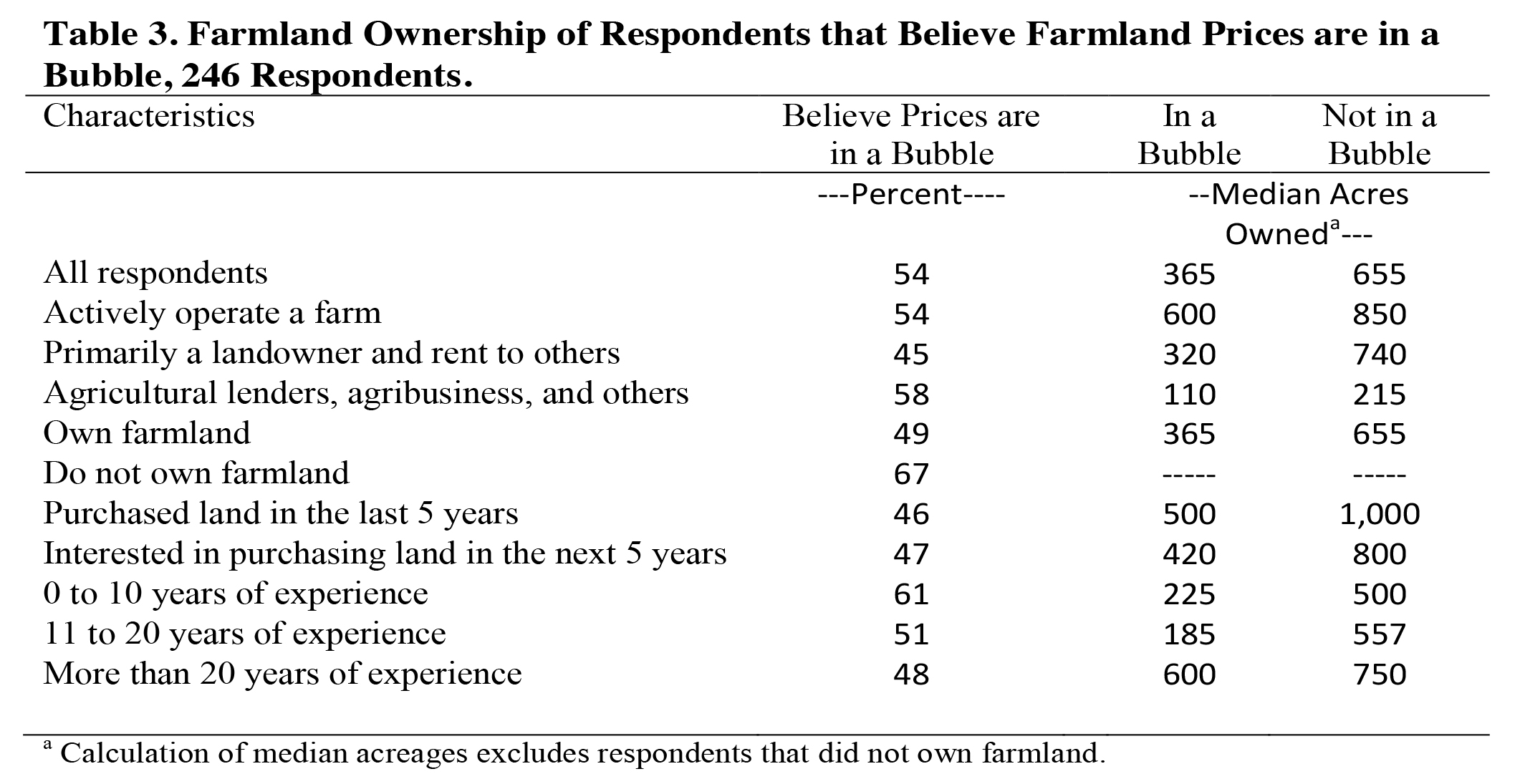
Table 3. Farmland Ownership of Respondents that Believe Farmland Prices are in a Bubble, 246 Respondents.
The last two columns of Table 3 show the median acres owned by each of the various groups depending on whether they felt that farmland prices were in a bubble. For example, 45percent of individuals who considered themselves primarily landowners that rented their farms to others,felt prices were in a bubble. The median acreage owned by those that felt the market was in a bubble was slightly less than half of those that felt the market was not in a bubble (320 acres as opposed to 740 acres). Across all groups, those who believed prices were in a bubble tended to own far fewer farmland acres. For nearly every group, those that felt prices were not in a bubble tended to have a median ownership of roughly twice those that felt the market was in a bubble.
When one examines the opinion as to whether farmland prices are in a bubble against the experience in farming,an interesting result emerges (Table 3). Here,one can see that those with less experience in farming tend to be slightly more likely to view farmland prices as in a bubble. As one would expect, those with less experience also tend to own less farmland.
Attitudes toward Valuation
Respondents were asked a series of questions regarding farmland valuation. The first series of questions introduced them to a hypothetical piece of farmland which would serve as the basis for several questions. The farmland was described as 80 acres with average quality soils and a yield production capability of 165 bushels of corn per acre under normal rain-fed conditions. The farmland description was written without an attached geographic location; rather,it was described solely on the basis of its size and yield potential. Respondents were then asked the following questions:
- What would you estimate this farmland to be worth today, in other words, what would you be willing to pay for this farm today ($s per acre)?
- What would be your estimate of the annual cash rental rate for this farm ($s per acre)?
- If you operate the above farm how much would you expect to earn annually after subtracting your estimate of the annual cash rent and cash operating expenses such as fertilizer, seed, chemical, fuel, etc. ($s per acre)?
Respondents were also given a chance to indicate that they would not purchase the farm at any price and opt out of the question and approximately 5 percent did so. The summary of the responses to the valuation questions are shown in Table 4.
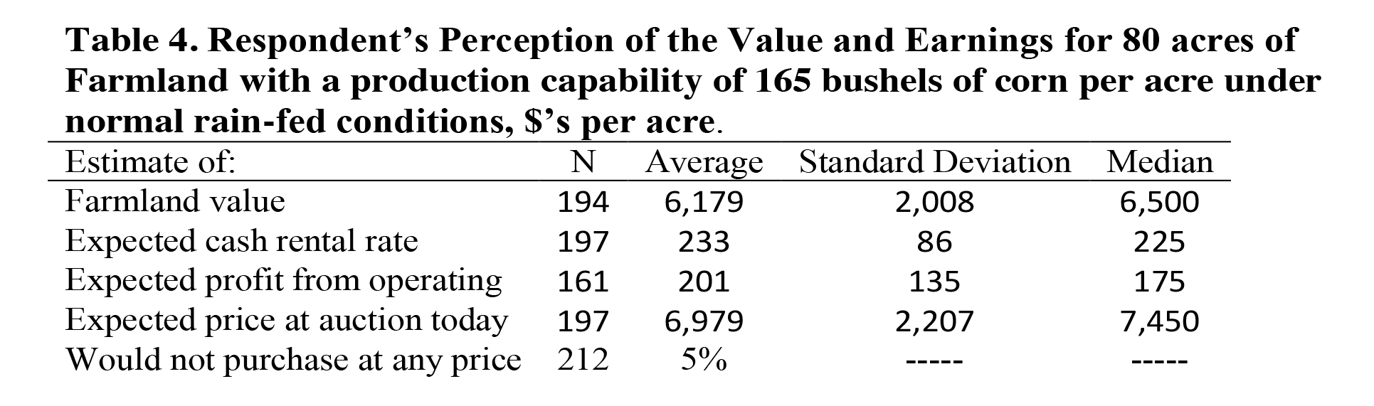
Table 4. Respondent’s Perception of the Value and Earnings for 80 acres of Farmland with a production capability of 165 bushels of corn per acre under normal rain-fed conditions, $’s per acre.
On average, the 194 respondents that answered the question placed a value of $6,179 per acre on the hypothetical farmland (Table 4). The median value was slightly higher, $6,500 per acre. The variability of the responses to this question was substantial, with the standard deviation of the responses at approximately $2,000 per acre. Indeed, a one standard deviation range around the mean would include prices from roughly $4,171 to $8,187. This wide range of possible outcomes is consistent with substantial amounts of uncertainty regarding the ultimate value of the farm, creating the potential for very large changes in the price of farmland.
In terms of income production, on average, the respondents expected that this farm would have a cash rental rate of $233 per acre. Again, the standard deviation was large relative to the mean. In this case,the standard deviation was 37percent of the mean, a slightly larger percentage than in the case of the land value. This result again highlights the wide range of views about the income production potential of the farm.
On average, respondents expected that if they operated a farm with these characteristics they would earn an expected profit after cash costs (including cash rent) of $201 per acre. Not surprisingly, it was clear that there was even greater variability for this value than either the value or rental rate question. Additionally, fewer respondents chose to answer the question about the expected profit that would be obtained by operating the farm, likely reflecting uncertainty over its value.
The results suggest that there is a wide range of opinions regarding values and income. There are several things that can be concluded from the variability. First, it is somewhat reassuring that respondents have widely differing views over both earnings and values. This is reasonable. One might be more concerned if the view on income was relatively homogeneous, but value estimates were variable. This would be one indication that value and income expectations were disconnected, however,this does not appear to be the case. Second, the wide range of value estimates should make for an active and liquid market. Clearly, there are some individuals with optimistic outlooks and others with more pessimistic views. This should facilitate the function of the market. Third, the wide extremes create the potential for substantial price swings in the market. Given the distribution of estimates, one should not be surprised when high prices are observed in the marketplace, both in terms of rents and farmland prices.
Someone Else will Pay More
Respondents were asked to estimate what they believed that this farmland would sell for at auction. Consistent with the general concern that the market was in a bubble, 65 percent of the respondents felt that their estimate of value was less than the prices in the market. On average, they placed the auction value at nearly $7,000 per acre (Table 5). In other words, most felt that someone else would be willing to pay more for the farm than their own estimate of value. In all but four cases, there was another respondent in the survey that felt the farm was worth at least what another respondent estimated its auction price to be.
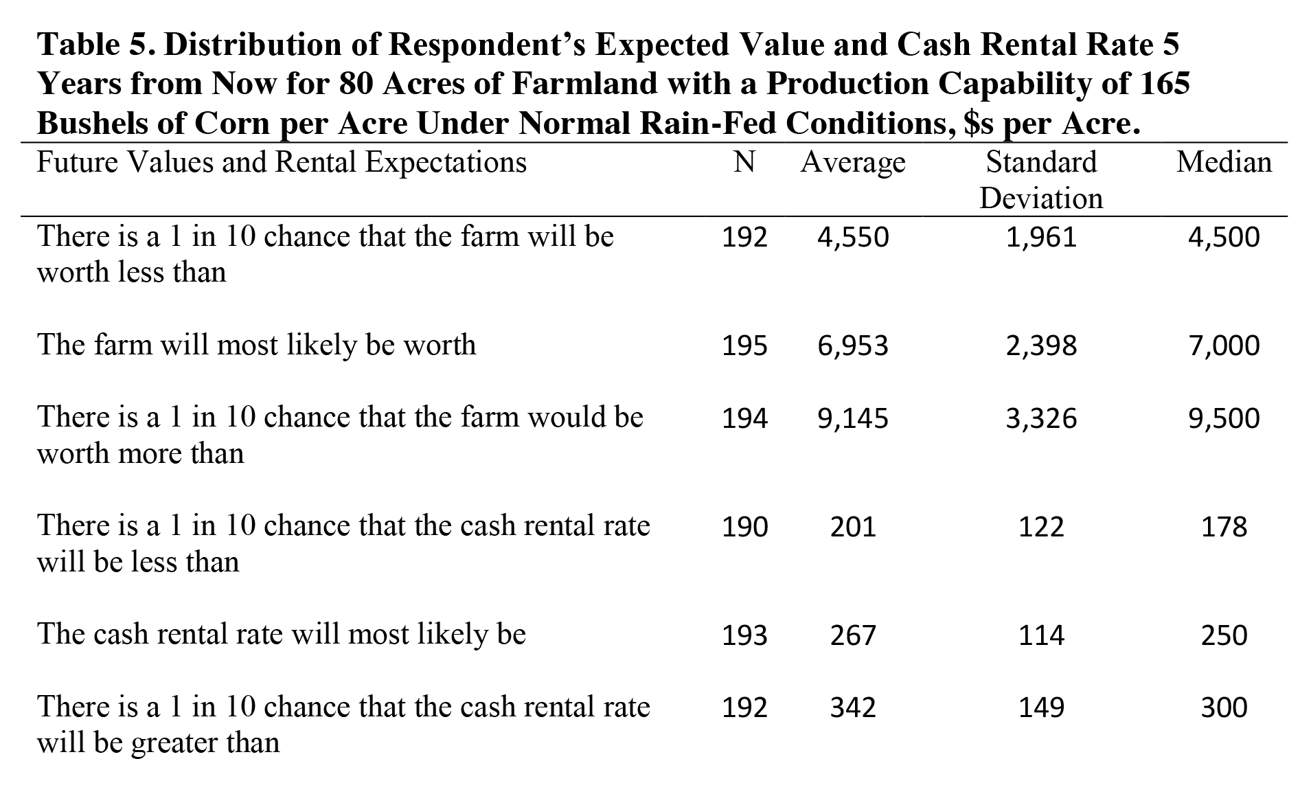
Table 5. Distribution of Respondent’s Expected Value and Cash Rental Rate 5 Years from Now for 80 Acres of Farmland with a Production Capability of 165 Bushels of Corn per Acre Under Normal Rain-Fed Conditions,$s per Acre.
The distribution of value and auction estimates is further illustrated in Figure 7. Here, the respondents are shown along the horizontal axis and their estimates of the value of the farmland are connected in a line arranged from low to high. What each individual estimated that the land would sell for at auction is shown with a triangle marker. This figure highlights the wide range of estimates that respondents had for the farmland. Nearly half of the respondents placed a value on the farmland greater than $6,500 per acre. Twenty percent of respondents felt that the farm was worth at least $8,000 per acre. On the other hand, 20 percent felt that the farm was worth $4,000 per acre or less.
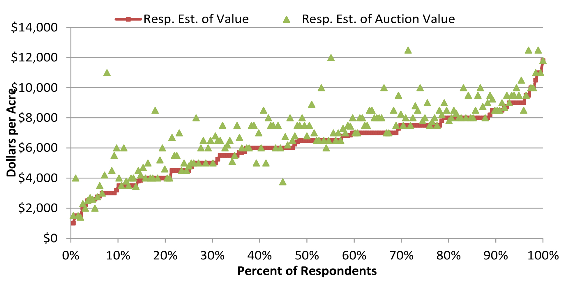
Figure 7. Respondent’s Estimates of their Value and the Auction Price of 80 acres of Farmland with a Production Capability of 165 bushels per acre of Corn under Normal Rain-Fed Conditions.
Value-to-Rent Relationship
On balance, the respondents are placing a high value on farmland relative to current rental rates. Calculated at the median and average estimates of value and rent, the value-to-rent ratio is 28.8 and 26.5 respectively. As noted previously, value-to-rent ratios of this magnitude are certainly high in the context of farmland pricing over the last 40 years. Today respondents appear to feel that ratios of this level are acceptable in the farmland market.
To further analyze the value-to-rent relationship, each respondent’s estimate of the value of the farmland was compared to the estimate of the cash rental rate. Figure 8 shows the distribution of the value-to-rent ratios. The frequency distribution can be read off of the left axis and the cumulative distribution off of the right axis. The most common value-to-rent ratio falls between 22.6 and 25. This would represent a capitalization rate between 4 and 4.4 percent.

Figure 8. The Distribution of the Value-to-Rent Ratio, 192 Respondents.
Very few respondents provided estimates that would place the value-to-rent ratio at less than 22.5. Roughly 80 percent estimated values that resulted in a multiple greater than 22.5 or a capitalization rate less than 4.4 percent. At the upper end of the range, almost 35 percent of the multiples were greater than 30. This represents a capitalization rate of less than 3.3 percent, which again is relatively low. Surprisingly, about 25 percent of respondents provided a rent-price combination that produced a multiple in excess of 32.5. Normally, one would accept such a low capitalization rates under the assumption that earnings were likely to grow in the future. This is particularly true in this case as the cash rental rates are gross rates and have no ownership expenses subtracted from them. If these were subtracted, the capitalization rate would fall even further.
The previously discussed value-to-rent ratio was calculated from what participants felt the land was worth to them and what they felt the cash rental rate would be. Recall that many participants felt that the farmland would sell for a higher price at auction. If one calculates the value-to-rent ratio off of the estimates of auction prices as opposed to what participants would be willing to pay for the farmland, the value-to rent ratios increase to very high levels. At the median values, the value-to-rent ratio would be 33,and at their means,the ratio would be 30, both very high levels in the context of history.
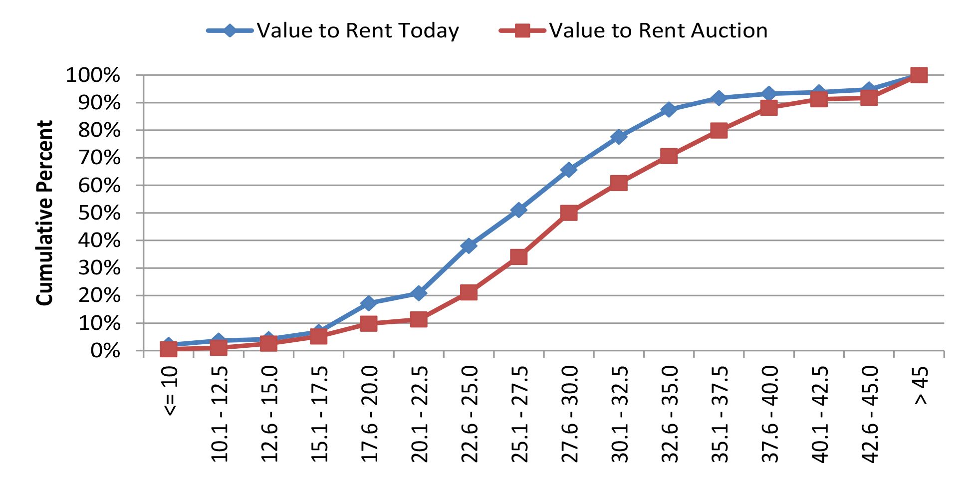
Figure 9. Cumulative Distributions of the Value-to-Rent Ratio Calculated Based on Respondents Estimates of Value and Auction Prices, 194 Respondents.
Figure 9 compares the cumulative distribution of value-to-rent ratios calculated from the respondents estimates of value and those calculated based upon their estimate of what the farm would sell for at auction. This chart provides a slightly different perspective on the market. Here, 50 percent of the respondents estimate that the value-to-rent multiple is in excess of 30; whereas,under their own estimates of value,only 35 percent would estimate a multiple this large. This chart may suggest that many participants feel that the value-to-rent multiple should likely fall from its current levels. If this were to happen, either rents would have to increase further relative to values or values would have to fall relative to rents.
Future Values and Incomes
In order to gauge whether respondents felt that land prices were likely to continue to increase, they were asked what they expected the farmland to be worth five years in the future. On average they expected the farmland to continue to appreciate, placing the most likely price in five years at $6,953 per acre (Table 5). This represents a 12.5 percent increase over their average estimate of current values. This is a relatively modest increase given that it would occur over a five-year period,and many states recently have seen annual increases in excess of 12.5 percent per year.
With respect to a range for land values, they felt that there was a 1 in 10 chance that prices for this land could be less than $4,550 and a 1 in 10 chance that they could be higher than $9,150. This represents a wide, but fairly symmetric view,of price risk around their most likely estimate. However, as one might suspect,the high/low most likely estimates varied considerably from respondent to respondent.
Figure 10 shows each respondent and their high, low, and most likely estimate of future land values. One can quickly observe from the figure that the individuals have very different opinions about the range in which they expect land trade in the future. Some see values with more downside than upside. Some see very wide ranges around the value expectations, while others believe values will likely be confined to narrow bands.
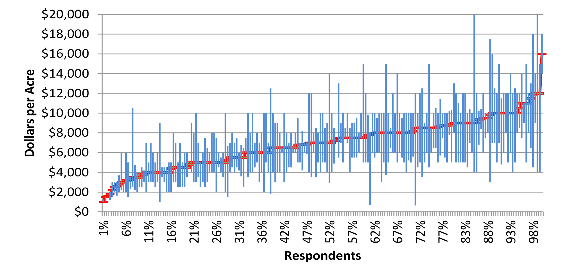
Figure 10. Respondents Estimates of the Most Likely, High, and Low Future Values of Farmland.a
a High and low estimates represent 1 in 10 chance that prices will be higher or lower than their estimate.
Where to in the Future? Multiples
At the means of the expected future land price and cash rental rate, the respondents expect that the value-to-rent multiple would remain at roughly 26. In other words, they expect that the increases in rental income to be capitalized at roughly the same rate as they feel is appropriate today. Based on a 26 multiple, the capitalization rate would be equal to 3.8percent (1/26).If one calculates the multiple based upon the medians, the expected multiple is 28 (7,000/250), which is slightly below the current multiple calculated off of median rent-to-value and implies a capitalization rate of 3.6percent.
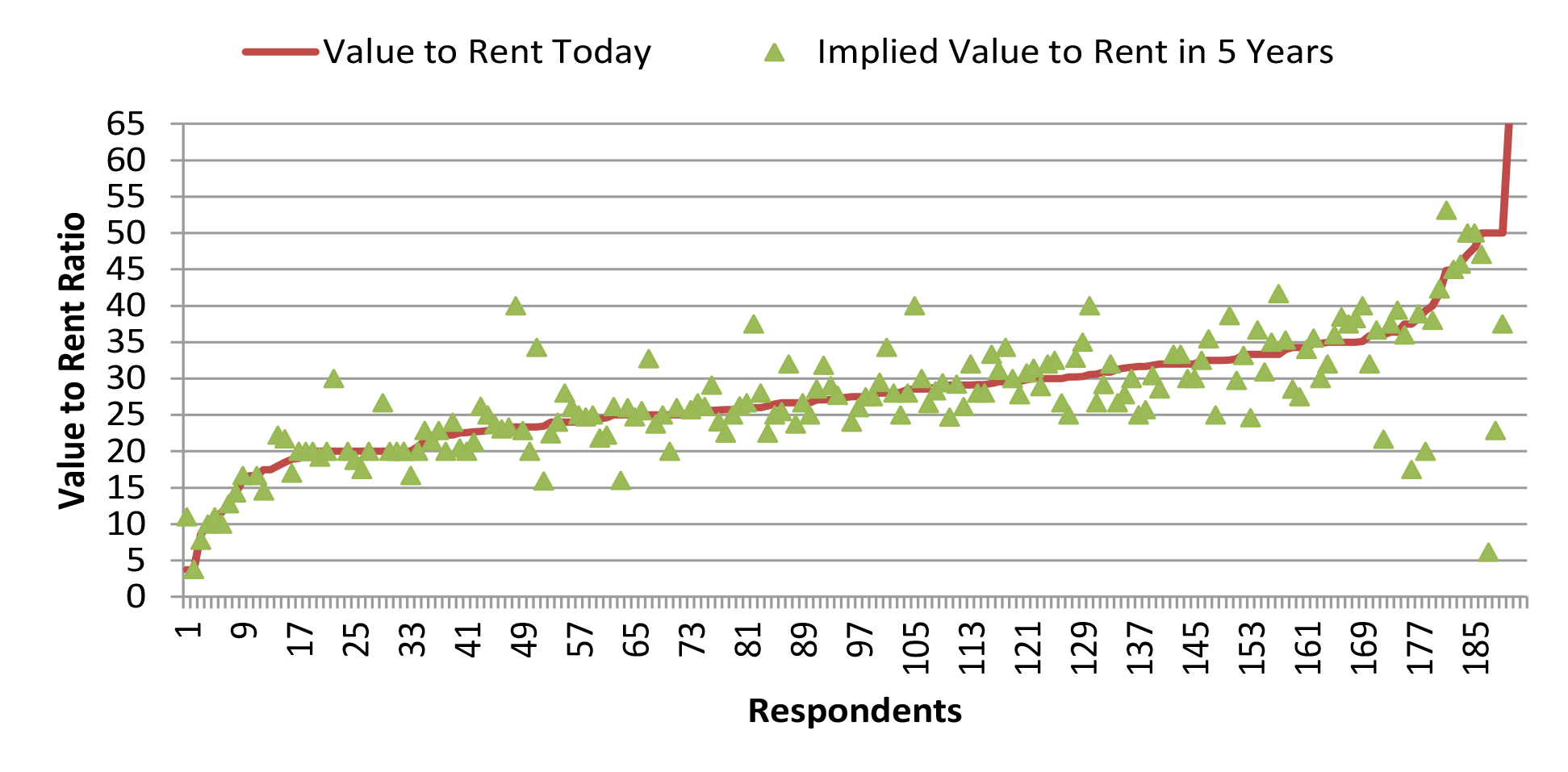
Figure 11. Comparison of Respondents’ Perceptions of the Value-to-Rent Ratio Today and 5 Years in the Future.
Figure 11 illustrates the distribution of the calculated multiples arranged along a line from low to high current multiples. The triangle markers show the calculated multiple for each respondent based on their future most likely land value and cash rent estimate. Triangles above the line indicate that the respondent produced a future land and rental estimate that resulted in a higher multiple thantheir estimate of current conditions. As can be seen from the figure, there is no clear view among the respondents as to whether the multiple should be increasing or decreasing in the future. In fact, 45 percent forecast a combination that would result ina multiple increase and 55 percent a decrease. This result lends further evidence to support the earlier claim that,on average,the respondents do not feel that the multiple will decrease dramatically in the future. However, the figure illustrates that many expect the multiple to change, with roughly similar amounts predicting decreases and increases.
The Link between Commodity Price Expectations and Values
Commodity prices play a key role in determining the amount of revenue that will be produced by a farmland investment. Respondents were asked to provide their most likely estimate of the average, high and low cash corn prices over the next five years. Again, the high and low price bands indicated prices with a 1 in 10 chance of occurring (Figure 12).
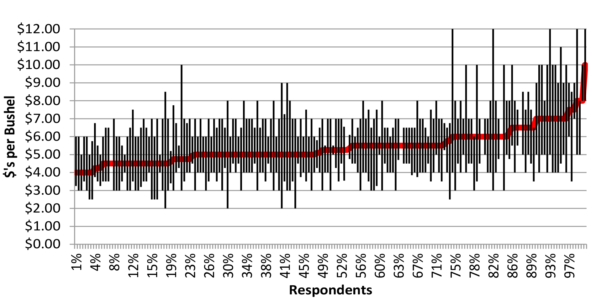
Figure 12. High, Low, and Most Likely Corn Price Forecasts, 189 Respondents.
On average, the respondents felt that cash corn prices would most likely average $5.41 per bushel over the next five years (Table 6). The median response was slightly lower at $5.25 per bushel. Using the average estimate of corn prices, the average yield of the hypothetical farm (165 bushels per acre), and the average expected cash rental rate would result in roughly 30 percent of expected corn revenue to be spent on cash rents.
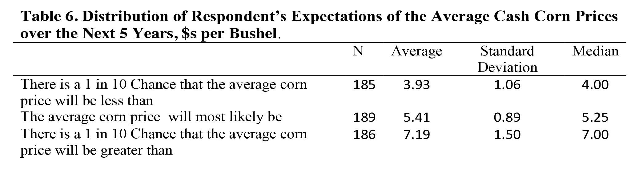
Table 6. Distribution of Respondent’s Expectations of the Average Cash Corn Prices over the Next 5 Years, $s per Bushel.
Perhaps the most surprising finding of the survey is shown in Figure 13, which shows the relationship between the farmland value estimates and the most likely estimate of corn price. One would expect that those who place higher values on farmland would also expect that corn prices would be high. However, one can quickly observe that,on balance,there is essentially no relationship between their expectations for corn prices and the estimate of farmland values. Indeed, the correlation between these two variables was close to zero, meaning that while some individuals with high land value estimates also feel that corn prices are likely to be quite high, others with high land value estimates feel that corn prices will be low.3
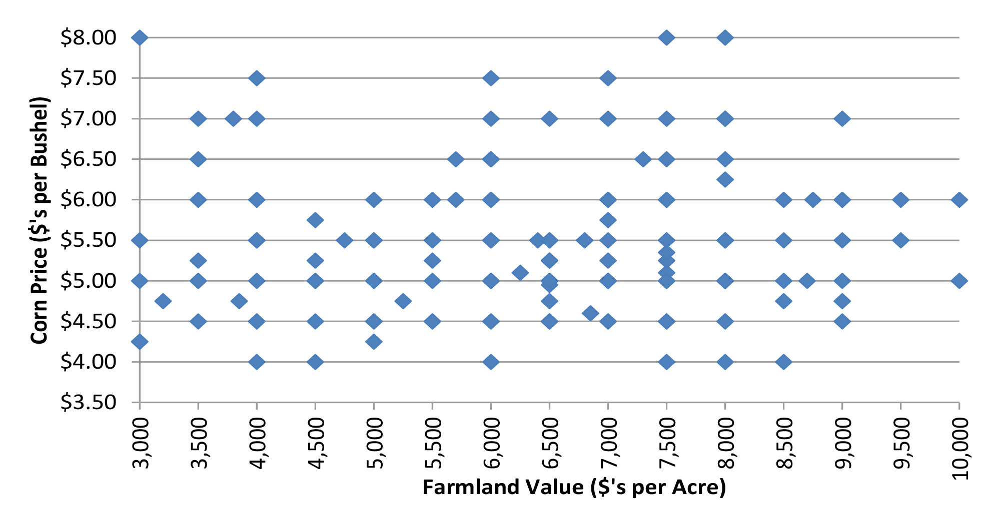
Figure 13. Relationship between Most Likely Corn Price Forecast and Estimate of Farmland Value.a a Figure shows respondents with land value estimates between $3,000 and $10,000 per acre.
Summarizing the Survey Results
Analysis of the data indicates that respondents do not expect the farmland multiple to continue to climb. Instead, they expect much more moderate increases in land values and cash rents over the coming five years. On average, over the next five years they expect land values and rents to edge up by a total of 12.5 percent and 14.5 percent respectively. This would indicate that most do not feel that the rapid recent appreciation experienced in the farmland market is likely to continue.
In fact, many respondents seemed to be concerned about the farmland market with slightly over half indicating that it was in a bubble. Although many felt that farmland was in a bubble, many were also interested in purchasing additional farmland in the coming years, perhaps providing support for the current values but a reluctance to follow values much higher than their current levels. On the other hand, those that felt prices were in a bubble tended to be much younger and have less experience in the farmland market, most likely the opposite of what one might expect in the case of a bubble. Further, those that did not feel the market was in a bubble tended to own significantly more acres of farmland than those that were concerned about a bubble.
In terms of the market conditions, the results of the survey are somewhat of a mixed bag. On average, respondents did not expect the value-to-rent multiple to expand dramatically in the future. This is encouraging in the sense that their estimates of value are likely consistent with their estimates of the income production of the farm. Surprisingly, the estimates of future corn prices showed almost no correlation with estimates of the value of farmland. This is a cause for concern. In order for incomes (rents) to increase in the future,one would expect that commodity prices would need to remain strong. It appears that some respondents’ views of commodity prices and farmland values are disconnected.
There was a great deal of variability among the estimates of the value of the farmland,and there was at least as much variability in the estimates of the cash rental rates. This indicates that the market is likely still searching for equilibrium prices after the dramatic crop price increases experienced in recent years. The supply of land available for purchase also appears to be limited. Nearly all of the respondents felt that the amount of farmland for sale was less than normal or about the same as usual.
The wide ranges in perceived value and relatively limited amounts of supply likely indicate that market transactions will be driven by those with the more extreme views of the value of farmland.In general, the purchasing capacity of the people at the upper end of the demand curve will likely be a key determinant of how high land values ultimately go. It is clear that there are a number of people with very bullish attitudes about the future of farmland prices. Where prices ultimately go will depend upon a number of factors, but until the supply of land offered to the market increases, it is likely that those at the upper end the demand curve will continue to push prices higher. How long this lasts will ultimately depend upon how these individuals’ expectations evolve.
Conclusions
There are many questions about the sustainability of the rapid price increases experienced in the farmland market. When placed in real values, the price increases experienced throughout much of the U.S. corn-belt are on par with those experienced in the 1970s, a period whose rapid price increases could not be sustained.
Many use the term bubble to indicate situations where asset prices undergo rapid expansions;indeed the 1970s farmland market conditions are frequently referred to as a bubble. Using the definitions of an economist, the identification of bubbles ex ante is very difficult,and true speculative bubbles are rare. It is unlikely that the current situation in the farmland market would satisfy the economic definition of a bubble.
While true bubbles are rare,it is also the case that rapid price escalations and declines do occur. Many of these situations are frequently associated with shocks that change underlying fundamental conditions. In some cases,it appears that market participants begin to focus less on market fundamentals and more on asset price changes. In the case of farmland, recent demand increases associated with biofuels and emerging economies and falling interest rates have served to spur rapid farmland price increases.
The level of farmland prices relative to its income generation is as high as at any time in history. For long-term sustainability, one would expect that these demand increases continue to materialize and interest rates remain low. Based on present prices,one must assume that investors expect these trends continue. A survey of market participant expectations revealed that many feel that the farmland market is currently in a bubble. However, the concerns were most strongly held by those that owned fewer acres and had less experience in the farmland market. Further, the respondents expect the rate of increase in farmland values to moderate going forward.
The survey provided some mixed evidence with respect to whether fundamentals are the focus of market participants. On average, they expect the relationship between income and values to persist in the future. This would be rational; they expect both income and values to increase. However, the relationship between expected future crop prices and farmland values was weak at best. One would expect that those with high farmland price expectations should expect high commodity prices and vice versa. There was little evidence that this was the case.
Given a limited supply of farmland available for sale, it is likely that sale prices will continue to be driven by those at the upper end of the demand curve. It is clear from the survey that there is a very wide range of views regarding the value of farmland and future economic conditions. It is yet to be determined how much purchasing power remains at the upper end of the demand curve. At this time,it appears that farmland prices are likely to remain strong.
Dramatic changes in underlying fundamentals like those experienced in the capital intensive agricultural sector present sector participants a significant challenge. If the changes are permanent or accelerate, capital assets will generate significant returns. Determining how high prices should adjust is an inexact science best left to market place participants. Problems in the adjustment process usually occur when market participants lose track of the underlying fundamentals, instead focusing on the price increases themselves. The limited evidence available on participant expectations shows some favorable signs as well as some suggesting that the connection between fundamentals and values maybe fraying.
The extent and impact of rapid asset price increases and decreases can be greatly magnified by financial leverage (Malkiel, 2010). Financial leverage allows investors to make larger bets on the direction of prices than would be possible if only equity is used to fund asset purchases. It also creates the potential for systematic liquidation of positions if lenders are forced to call loans and liquidate collateral as happened in the 1980s farm crisis.
To date, it does not appear that leverage is playing a significant role in the asset appreciation. This does not preclude a dramatic rise and collapse of farmland prices, but it does potentially limit the magnitude of the damage from capital misallocation. Given the potential impact of increasing financial leverage in a period of rapid asset price increases, it is important to monitor the leverage situation closely. While a lack of leverage does not rule out the possibility that prices could decline substantially in the future, it likely limits the damage that would be done to the sector if that were to occur.
1 Melichar (1979) used USDA estimates of unpaid labor and management whichapparently consisted of a flat percentage of total revenue in the sector. It appears that these series are no longer estimated by the USDA, so they remain in the total return. When interpreting this series it is useful to remember that these factors must be paid from the total return.
2 It is important to acknowledge that this series includes the return to unpaid labor and management, which if falling dramatically over recent times, could explain some of the reduction in returns.
3 The lack of a relationship between corn price expectations and land values was also explored with a regression analysis that controlled for factors such as interest rate expectations. Consistent with the chart, no significant relationship was found.
References
Barlevy, G. “Economic Theory and Asset Bubbles.” Economic Perspectives, Federal Reserve Bank of Chicago, 31:3(2007):44-59.
Buffett, W. Financial Crisis Inquiry Commission Staff Audiotape of Interview with Warren Buffett, Berkshire Hathaway, May 26, 2010. Transcribed by Santangel’s Review.
Dobbins, C.L. and K. Cook. “Indiana Farmland Market Continues to Sizzle.” Purdue Agricultural Economics Report, August 2011. http://www.agecon.purdue.edu/extension/pubs/paer/pdf/PAER8_2011.pdf
Duffy,M.D. “Iowa Land Values –All Historical Values 2011.” Available at: http://www2.econ.iastate.edu/faculty/duffy/documents/IowaLandValuesALLHistoricalValues2011.xls
Economic Research Service, U.S. Department of Agriculture, Farm Income and Balance Sheet Indicators, 1929-2010.
Garber, P.M. “Famous First Bubbles.” Journal of Economic Perspectives, 4:2(1990):35-54.
Gloy, B.A., M.D. Boehlje, C.L. Dobbins, C. Hurt, and T.G. Baker. “Are Economic Fundamentals Driving Farmland Values?” Choices, 26:2(2011).
Gloy, B.A., C. Hurt, M. Boehlje, and C. Dobbins. “Farmland Values: Current and Future Prospects.” Center for Commercial Agriculture, Research Paper, January 11, 2011. Available at: https://www.agecon.purdue.edu/commercialag/progevents/LandValuesWebinar/Farmland_Values_Current_Future_Prospects.pdf
Gloy, B.A., B. Allen, J. Lai, S. Li, Y. Liu, M. McKendree, J. Timberlake, D. Urick, H. Wendler. “Farmland Value Expectations and Influences: Evidence from the Field.” Center for Commercial Agriculture, Research Paper, May 2012.
Henderson, J. and M. Akers. “Farmland Values Rise with Crop Prices.” Survey of the Tenth District Agricultural Credit Conditions, Federal Reserve Bank of Kansas City, First Quarter 2012.
Henderson, J., B.A. Gloy, and M.D. Boehlje. “Agriculture’s Boom-Bust Cycles: Is This Time Different.” The Economic Review, Kansas City Federal Reserve Bank, 96:4(2011): 83-101.
Malkiel, B.G. “Bubbles in Asset Prices.” Princeton University, Center for Economic Policy Studies, CEPS Working Paper No. 200, January 2010.
Malkiel, B.G. “The Efficient Market Hypothesis and Its Critics.” Journal of Economic Perspectives, 17:1(2003):59-82.
Melichar, E. “Capital Gains Versus Current Income in the Farming Sector.” Paper presented at the Annual Meetings of the American Agricultural Economics Association, August 1, 1979.
Shiller, R.J. “Speculative Prices and Popular Models.” Journal of Economic Perspectives, 4:2(1990):55-65.
Shiller, R.J. “From Efficient Markets Theory to Behavioral Finance.” Journal of Economic Perspectives, 17:1(2003):83-104.
Siegel, J.J. “What is and Asset Price Bubble? An Operational Definition.” European Financial Management, 9:1(2003):11-24.
Stiglitz, J.E. “Symposium on Bubbles.” Journal of Economic Perspectives, 4:2(1990):13-18.
![]()
![]()
![]()
![]()
![]()
TEAM LINKS:
PART OF A SERIES:
RELATED RESOURCES
UPCOMING EVENTS
We are taking a short break, but please plan to join us at one of our future programs that is a little farther in the future.