January 1, 2014
Farmland: Is it Currently Priced as an Attractive Investment?
![]()
![]()
![]()
![]()
![]()
Introduction
Farmland comprises the vast majority of farmers’ asset base and personal wealth; USDA balance sheet data indicate that farmland accounts for approximately 85% of the value of the total assets in production agriculture (USDA-ERS). This percentage has been increasing during the past decade in large part because of the dramatic increase in farmland prices. U.S. farmland prices have increased 37% during the last 5 years, and in real terms prices have risen 7-10 percent annually in Corn Belt states like Iowa and Illinois (Gloy, 2013). The recent dramatic increase in farm real estate prices has attracted interest from the broader investment community in farmland as a component of their investment portfolio as illustrated by TIAA-CREF’s recent acquisition of the farmland portfolio of Westchester, a large farmland realtor and investment company with properties throughout the U.S. Similar investment interest is reflected by the numerous articles on farmland investing on websites such as www.bankrate.com (Gustke, 2013) www.financialsense.com (Robinson, 2013), www.forbes.com (Forbes, 2013), and www.beta.tool.com (Lube, 2013).
Concern is being expressed by many that farmland prices will become higher than justified by the fundamentals, and result in what we will later recognize as a bubble (Bowman, 2013; Watts, 2013). One justification for this concern is that previous research has established the tendency of the farmland market to over-shoot (Burt, 1986; Featherstone and Baker, 1987; Featherstone and Baker, 1988). So, from the standpoint of the literature and history, another bubble in farmland prices would not be a surprise.
Numerous previous studies of farmland prices and values have been completed as summarized by Moss and Katchova (2005). This analysis builds on and extends earlier work by positioning the farmland investment decision as an investment portfolio choice. The focus will be on the financial attractiveness of farmland as an investment. We will not attempt to assess the numerous non-economic arguments often made by farmers (and others) to justify the purchase of a particular parcel of farmland. Thus, our discussion will emphasize the risk, return, portfolio and inflation hedge characteristics of farmland in comparison to other common financial investments that one might make. It is also important to note that we will not focus on the operational details of managing and maintaining farmland which may present significant challenges (and opportunities) requiring specialized farm management expertise.
To frame the farmland as an investment choice analysis, the commonly accepted income capitalization model of asset valuation is used. The constant growth present value model provides the theory behind this analysis procedure. In this model the return to an asset at the current time (R0) is expected to grow at rate g indefinitely, and the required rate of return is r (also constant into perpetuity), leading to the following present value equation.
Solution to the infinite series of equation (1) yields the constant growth model (2):

From equation (2) we can derive the common investment analysis metrics of cap rate (R1/Value) and the inverse of the cap rate, the value (or price) to earnings (P/E) ratio or multiple. In equation (2), the capitalization rate is the difference between the required rate of return (r) and the anticipated indefinite constant growth rate (g). The P/E multiple will increase as the difference r-g declines, which means that reducing the required rate of return, or increasing the expected long-term grown in earnings are the two factors that will increase the multiple.
P/E ratios for stocks are compared to the price to earnings multiple (P/rent) for farmland in this paper. The P/E ratio is computed by dividing market value per share for a particular stock or group of stocks by the appropriate earnings per share (EPS). Historical or expected earnings per share can be used in the computation. P/E ratios reported typically use historical earnings per share to compute the ratio. The average market P/E ratio for stocks is 15 to 20; however, it is important to note that the average P/E ratio does vary across industries. In general, a high P/E ratio indicates that investors anticipate higher growth of earnings in the future. These results are augmented by econometric estimates of the beta (β), a fundamental relative risk metric, for farmland, gold, and housing assets; and the relationship between farmland values and expected and unexpected inflation.
Data
For the P/E ratio analyses data on a cash rent and farmland price series for West Central Indiana from 1960 to 2013 were used. The 1974 to 2013 data were obtained from the annual Purdue survey of Indiana cash rent and farmland values; the most recent survey is reported in Dobbins and Cook (2013). To obtain estimates from 1960 to 1973, the Purdue survey data were extended back using USDA data.
The reason for using West Central Indiana farmland prices and cash rent is that budgeted “actual” owner operator returns using actual yields is available to determine incomes or returns. Tippecanoe County average yields of corn and soybeans, season average prices of corn and soybeans, Purdue Crop Budget costs (e.g., Dobbins et al., 2013), Environmental Working Group data for government payments for the years available (budgeted government payments for earlier years), and a 50-50 corn-soybean rotation were used to compute historical owner operator returns. Owner-operator returns are the most important factor driving the cash rental market which is the best indicator of the return to land (albeit a measure of return before landlord costs such as property taxes are subtracted).
Inflation indices and interest rates on 10-year Treasuries are gathered from the Federal Reserve Bank of St. Louis (www.research.stlouisfed.org/fred2/). The implicit price deflator for personal consumption expenditures is used to measure inflation. The S&P data were obtained from various web sites (www.multpl.com; www.irrationalexhuberance.com).
For the econometric estimates of long-run risk, return, and inflation hedge characteristics of farmland, data from 1911 to 2012 for returns to Iowa farmland (cash rent and capital gains), S&P 500 returns (dividends and capital gains), gold, housing, and inflation are used. Iowa farmland data are from USDA surveys; S&P 500 data, CPI inflation, and housing price changes are from Robert Shiller.1 Gold prices are London gold fixing prices. We use continuous annual percentage rates.
Results
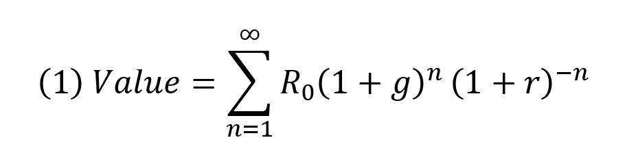
The P/rent ratio for West Central Indiana has an average value of 17.9 over the 53 year period from 1960 to 2013 with a high of 31.8 reached in the last year of data (2013) and a low of 11.1 in 1986, which was perhaps the bottom of the valley after the bubble of the 1970s and 1980s (Figure 1). At the peak of this bubble, the P/rent multiple reached a high of just over 20 from 1977 through 1979. The P/rent multiple subsequently dropped to the teens in the early 1980s, and down to its low in 1986. The rise from around 15 in 1976 into the 20s and down to 11.1 in 1986 corresponds exactly to what is viewed as the bubble in farmland prices and one of the more difficult periods for agriculture in modern history. It is within this historical context that the rise in the P/rent ratio from the upper teens in the later 1990s to last year’s survey value of 31.8 is of alarm.
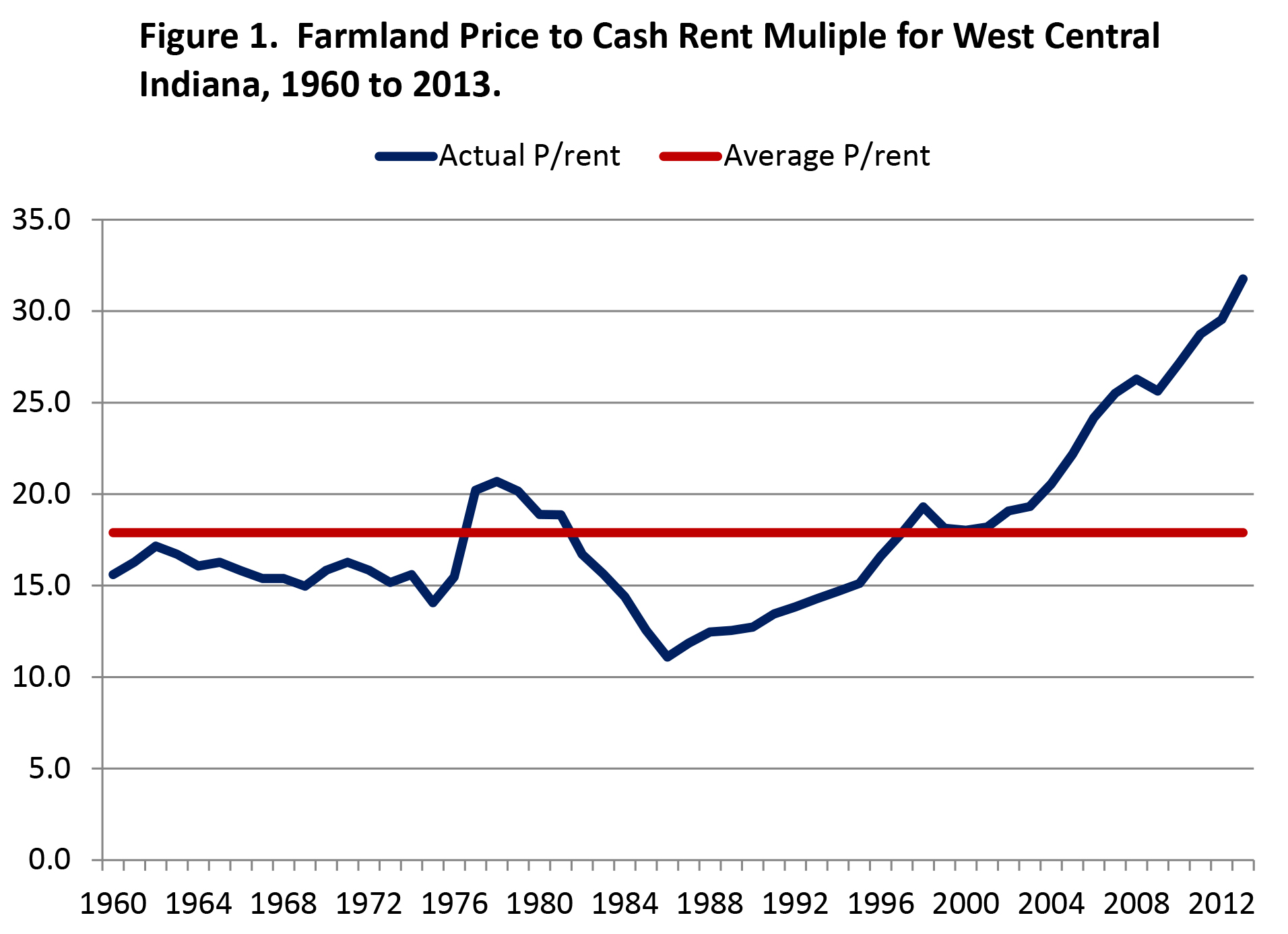
Figure 1. Farmland Price to Cash Rent Multiple for West Central Indiana, 1960 to 2013.
Interest Rates
Falling interest rates likely help explain the recent rise in the P/rent ratio. Ten-year US Treasury average annual interest rates have fallen fairly steadily from a peak of 13.1% in 1981 to approximately 2.0% in 2012 and 2013. The required rate of return by farmland investors would be higher than the 10-year U.S. Treasury interest rate due to a risk premium, which is expected to be at least as large as the premium of the farm borrowing rate over the 10-year U.S. Treasury rate which is 1.99%.2 If farmland market participants have required rates of return for farmland that follow the 10-year Treasury rate (plus a constant risk premium), then the time series pattern shown by the 10-year Treasury rate provides an indication of the direction of change in the discount rate in the constant growth model.
The reciprocal of the 10-year Treasury interest rate tracks the increase in the farmland P/rent ratio from 1985 to 2010 (Figure 2). In the period from 1960 to 1985 there is not an obvious connection between the P/rent ratio and the 10-year Treasury interest rate. Also, in the last several years the reciprocal of the 10-year Treasury rate has risen much faster than the P/rent ratio. If the recent very high P/rent ratios are caused by the recent extremely low interest rates (which results in a high re
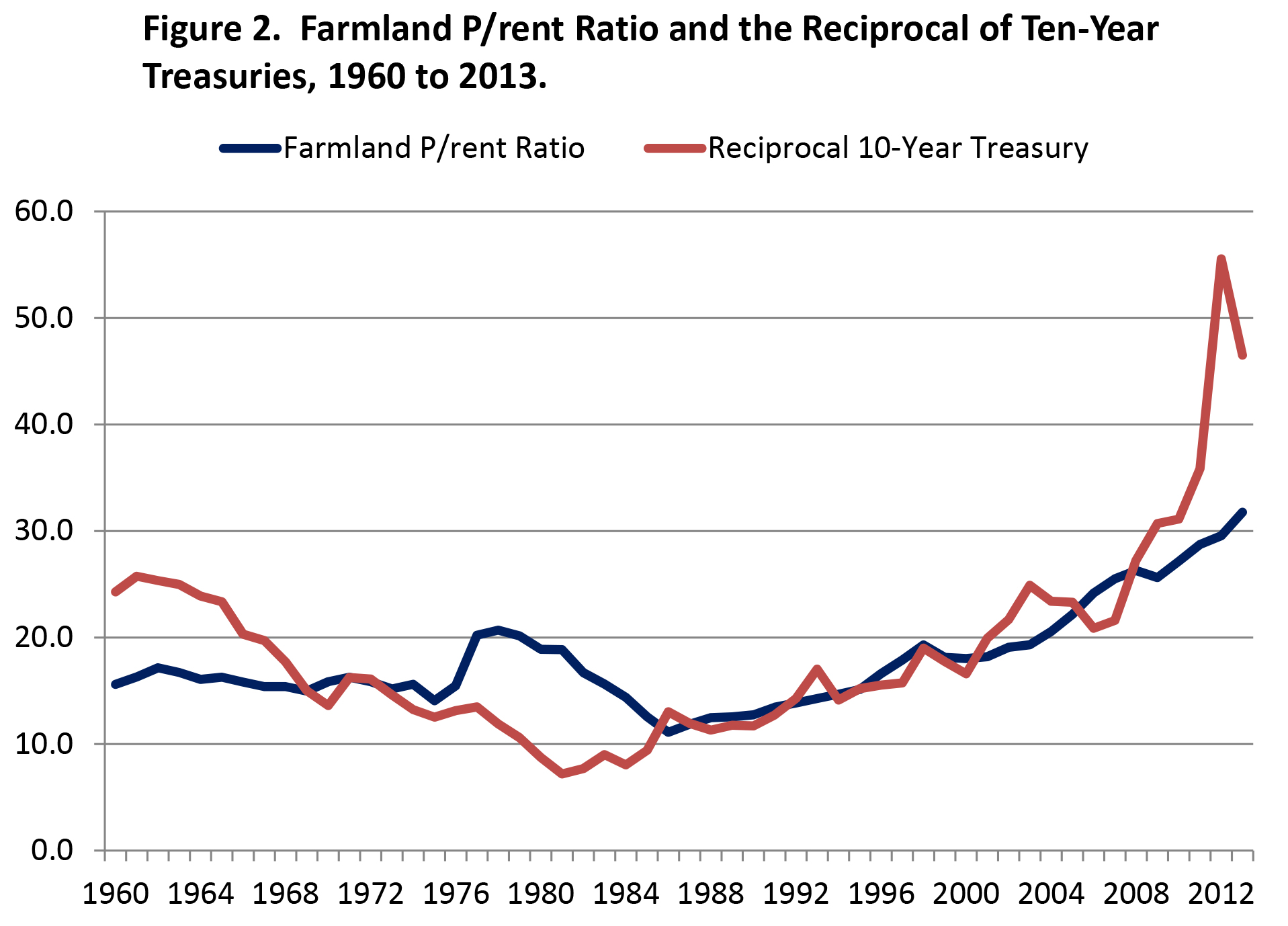
Figure 2. Farmland P/rent Ratio and the Reciprocal of Ten-Year Treasuries, 1960 to 2012.
ciprocal), then the implication is that the market expects relatively low rates to continue over the long term. Interest rate futures markets and a positive slope in the Treasury yield curve have been predicting rising interest rates for the last two years, and even though this has not occurred,3 it is reasonable to question the long-run persistence of low interest rates required as the fundamental to justify high P/rent ratios.
Equity Investment Comparisons
We compare the P/rent ratio to stock market indices to obtain insight into the comparative attractiveness of farmland as an investment. Figure 3 shows the P/E ratio for the S&P 500 and the P/rent ratio. The average P/E ratio for the S&P 500 for the period at 18.2 is relatively close to the 17.9 average for the P/rent ratio for farmland. With the exception of 1995 and 1997, the P/E ratio was higher than the P/rent ratio from 1986 to 2003. Since 2003, except for 2009 which exhibited a very high P/E ratio for stocks,4 the P/rent ratio for farmland has been higher than the P/E ratio. In addition to being relatively high, the P/rent ratio has exhibited an upward trend in the last ten years. The current P/rent ratio of 31.8 is well above the average P/E multiple, and very unattractive compared to the 2004 to 2013 P/E ratio.
Figure 3. Farmland P/rent Ratio and S&P 500 P/E Ratio, 1960 to 2013.
There are shortcomings in comparing P/rent and P/E ratios. Cash flow received by a stock investor is the dividend on the stock, not the earnings. The percentage of earnings per share (EPS) paid out as dividends varies from company to company, ranging from zero to over 100 percent. Historically, the dividend payment ratio for the S&P 500 has averaged about 55%. In recent years, this ratio has been closer to 30%. An alternative metric would be to compare the P/rent ratio for farmland to the price/dividends (P/D) ratio for stocks. Dividends are of course smaller than earnings, so price/dividend (P/D) ratios are higher than P/E ratios. The prices of shares of stock in companies reflect both the dividend payout and the effect of retention on expected growth. The effect of changing payout and retention rates is masked when looking at the P/E ratio at different times and comparing different companies. Because of these confounding factors, comparing P/D ratios of individual companies or even stock indexes to farmland is probably of limited value because of the extreme variation in dividend payout policies.
Growth in Farmland Returns
As previously indicated, the expected long-run future growth rate in farmland returns is one of the key variables in the constant growth model and is a major determinant of the P/rent ratio. Farmland market participants likely look at past growth in rent when anticipating future growth because it is human nature to use past experience when assessing the future. Thus, one would expect participants in the farmland market to be looking at past growth in returns along with current information about drivers of that growth to base their expectations.
Growth in cash rent (year-over-year continuous percentage change)5 and the 5- year moving average growth rate are shown in Figure 4. The mean growth in returns to land over the last 50 years has been 4.6%. The 5-year and 10-year moving averages of growth rates in cash rent have movements that are similar to the patterns shown in the farmland P/rent ratio (Figure 5). Extremely high growth rates in cash rent were experienced in the middle 1970s. The growth rates of course fell through the middle 1980s. The 5-year moving average smooths the year to year changes in annual growth and lags substantial increases and decreases in growth, but generally speaking follows the same pattern as the current growth rate in cash rent. While the 5-year moving average might be a good indicator of the optimism or pessimism of those in agriculture, it is hard to believe that farmland market participants expected long-term growth in the -5.0% range in the later 1980s, but surely the anticipated growth in the 1980s was lower than what it was in the mid-1970s. If market participants did have expectations following a moving average it would explain the markets tendency to over and under shoot. If recent growth in rent has been high, the moving average increases, and if the expectation of higher growth rate in rent follows, then the P/rent ratio would increase. The reverse would happen when rents fall. Thus, land values would be increasing or decreasing both because rents increase or decrease, and because the P/rent multiple increases or decreases.
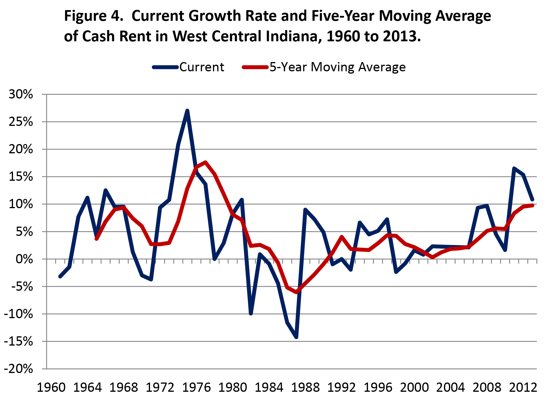
Figure 4. Current Growth Rate and Five-Year Moving Average of Cash Rent in West Central Indiana, 1960 to 2013.
The logic of farmland market participants’ expectations of growth following a moving average pattern is troublesome. When returns grow it is generally due to high crop prices. Long-run supply response might suggest slower growth would follow high growth, a contrarian view of growth, rather than believing that good times beget further good times.
Cyclically Adjusted P/Rent
Shiller (2005; 2013) uses a 10-year moving average for earnings (often labeled either P/E10 or CAPE) in order to remove the effect of the economic cycle on the P/E ratio. CAPE is an acronym for cyclically adjusted P/E. When earnings collapse in recessions, stock prices often do not fall as much as earnings, and the P/E ratios based on the low current earnings sometimes become very large (e.g., 2009). Similarly, in good economic times P/E ratios can fall and stocks look cheap, simply because the very high current earnings are not expected to last, so stock prices do not go up by as much as earnings. By using a 10-year average of earnings in the denominator of the P/E ratio, Shiller has smoothed out the business cycle. In Shiller’s calculations he also deflates both earnings and prices to remove the effects of inflation.
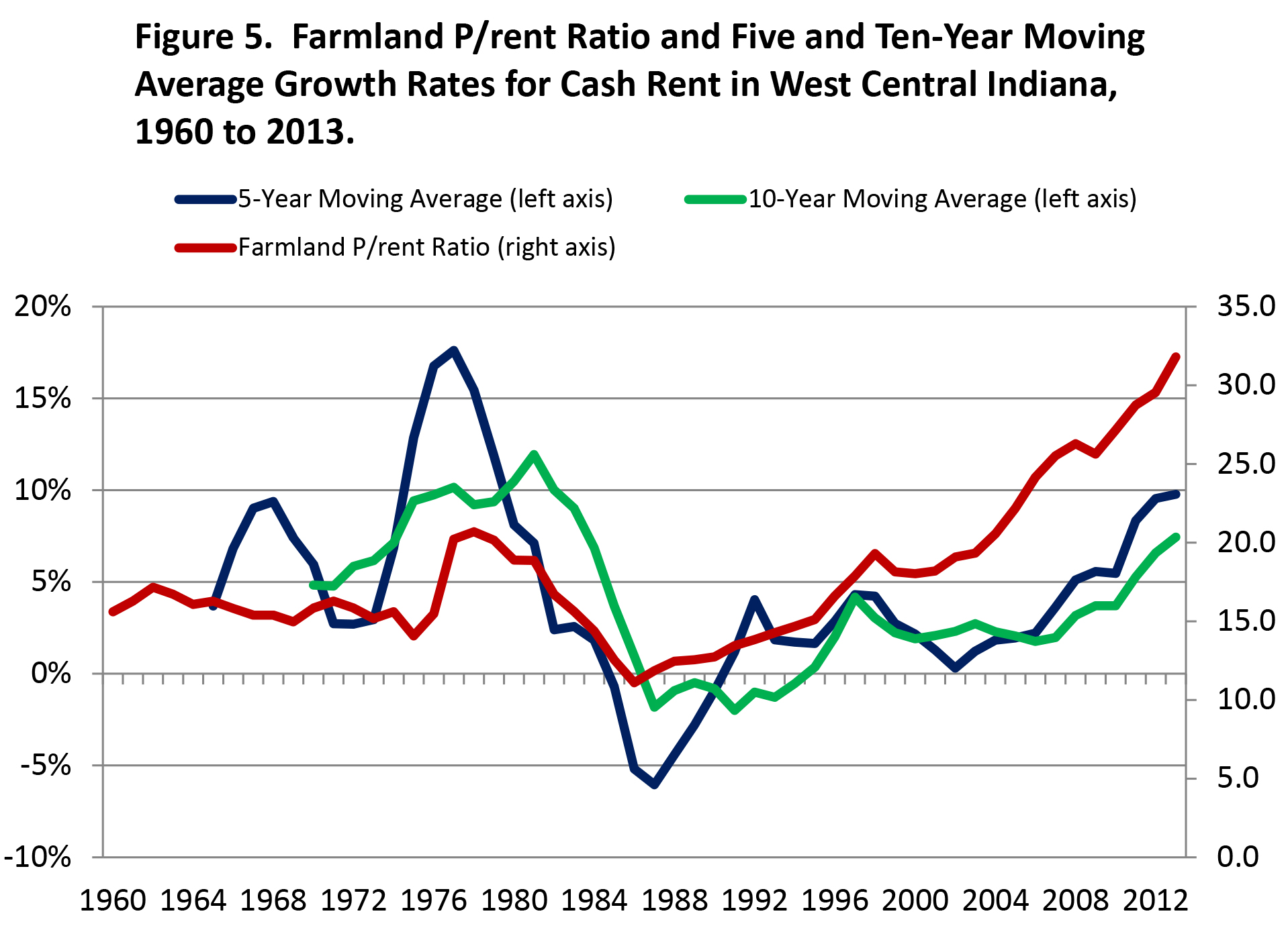
Figure 5. Farmland P/rent Ratio and Five and Ten-Year Moving Average Growth Rates for Cash Rent in West Central Indiana, 1960 to 2013.
The P/rent ratios reported thus far are the current year’s farmland price divided by cash rent for the same year. P/rent10 is modeled after Shiller’s cyclically adjusted P/E ratio. Cash rent and farmland prices are deflated, and then 10-year moving averages of real cash rent are calculated. The P/rent10 ratio is computed by dividing the real farmland price by the 10-year moving average real cash rent. A similar computation is done for 10-year owner-operator returns (P/00-10).
Figure 6 presents real land prices divided by 10-year moving average real cash rents and real owner operator returns as well as Shiller’s P/E10 ratio. The P/OO-10 fell through the first half of the 1970s when real returns grew faster than land values, increased from the high teens in the middle 1970s to 28.2 in 1977, and then fell to 6.8 in 1987. The P/OO-10 then increased steadily until it reached 37.6 in 2013. In the last two years, the P/rent10 ratio has risen substantially above the P/OO-10 ratio. Two points are evident from Figure 6. First, the P/rent10 ratio in 2013 has exceeded the peak of Shiller’s P/E-10 ratio during the dot.com bubble. Second, the relationship between the P/rent10 ratio and the P/OO-10 ratio suggests that producers are not bidding all of the increases in owner operator returns into cash rents. Producers may be expecting owner operator returns to decline, which would make it difficult to maintain high cash rents. However, this relationship could also be explained if one expects cash rents to adjust slowly to changes in operator returns. Historically, there have been times when cash rents were slow to adjust.
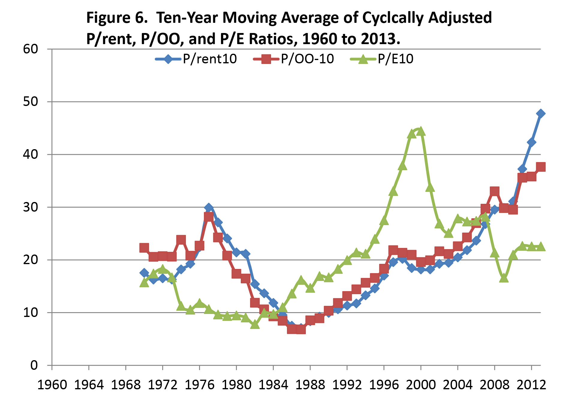
Figure 6. Ten-Year Moving Average of Cycically Adjusted P/rent, P/OO, and P/E Ratios, 1960 to 2013.
Shiller (2005; 2013) shows the relationship between the P/E10 ratio and the annualized rate of return from holding S&P 500 stocks for long holding periods. In general, his results show that the higher the P/E10 ratio at the time of purchase, the lower the resulting 10-year returns. The farmland and cash rent data from 1960 to 2013 are used to compute 10-year and 20-year annualized rates of return (computed as the sum of the average of cash rent as a fraction of the farmland price each year plus the annualized price appreciation over the holding period). The results for farmland show a negative relationship similar to that exhibited in Shiller’s stock data. The 10-year holding period returns for farmland show a strong negative relationship (Figure 7), the higher the P/rent10 (farmland price divided by 10-year moving average of cash rent) at the time of purchase, the lower the resulting 10-year rate of return. The 10-year holding returns range from a slightly negative rate of return to 20%. The 20-year holding period returns also exhibit a strong negative relationship with the P/rent10 ratio (Figure 8). The 20-year holding returns range from 6 to 14%. The P/rent10 levels in the last 4 years are literally off the chart, much higher than any P/rent10 value for which we have a 10- or 20-year return.
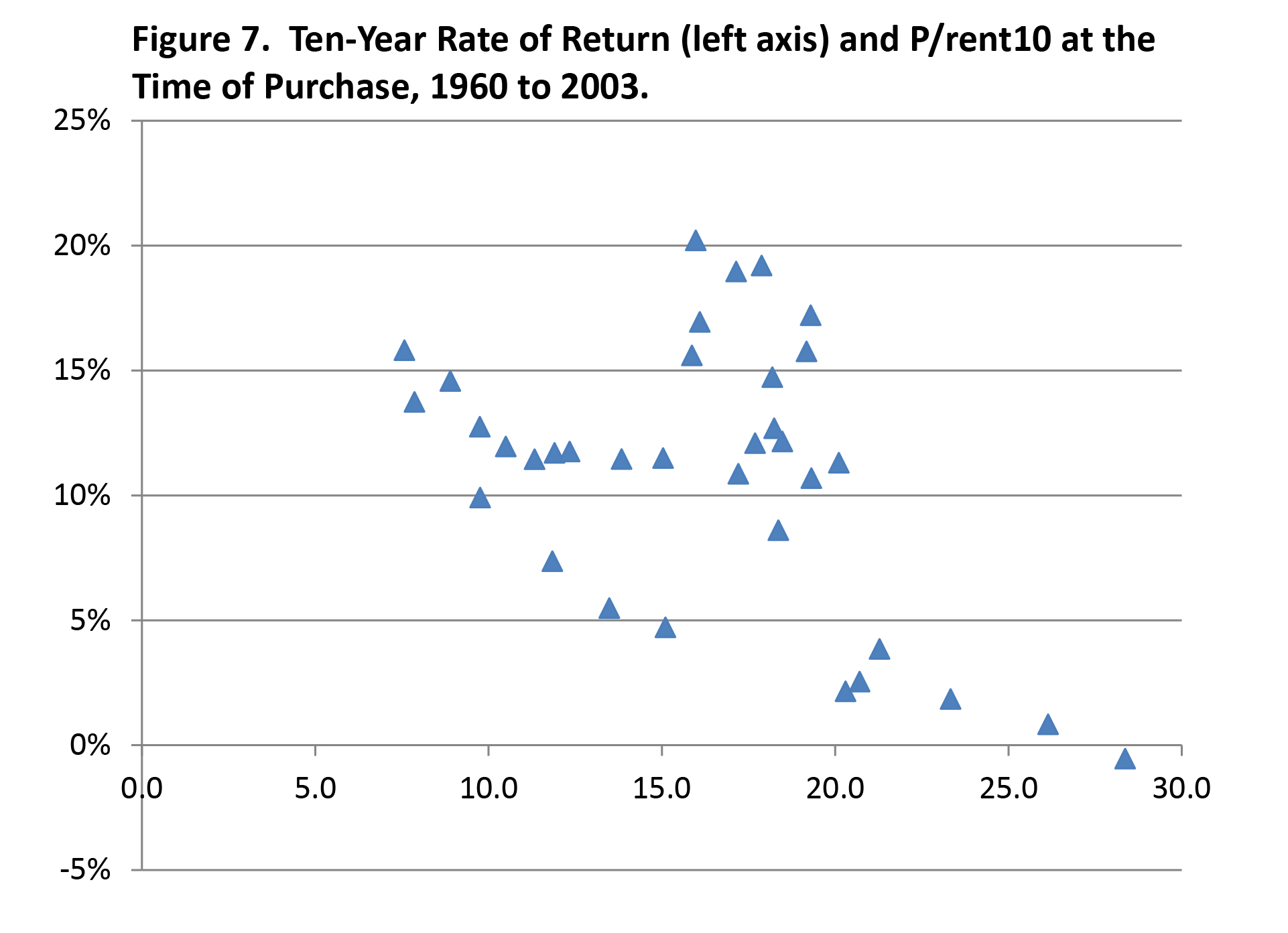
Figure 7. Ten-Year Rate of Return (left axis) and P/rent10 at the Time of Purchase, 1960 to 2013.

Figure 8. Twenty-Year Rate of Return (left axis) and P/rent10 at the Time of Purchase, 1960 to 1993.
Long-Term Risk, Return, and Inflation Hedge
Finally, the risk, return and inflation hedge characteristics of Iowa farmland are presented to investigate the attractiveness of farmland as a portfolio investment. The means, range and correlation of the key variables used in the econometric estimation are shown in Table 1. Iowa farmland has a mean return of 10.7% that is comparable to the S&P 500 mean return of 9.0%. The 1.7% higher mean rate of return is not significant given that landlords normally have to pay some expenses out of cash rent (landlords usually pay property taxes and sometimes pay other expenses such as tile upkeep and lime). The conventional wisdom that farmland has a competitive rate of return, comparable to stocks, appears to be supported by the 101 years of data.
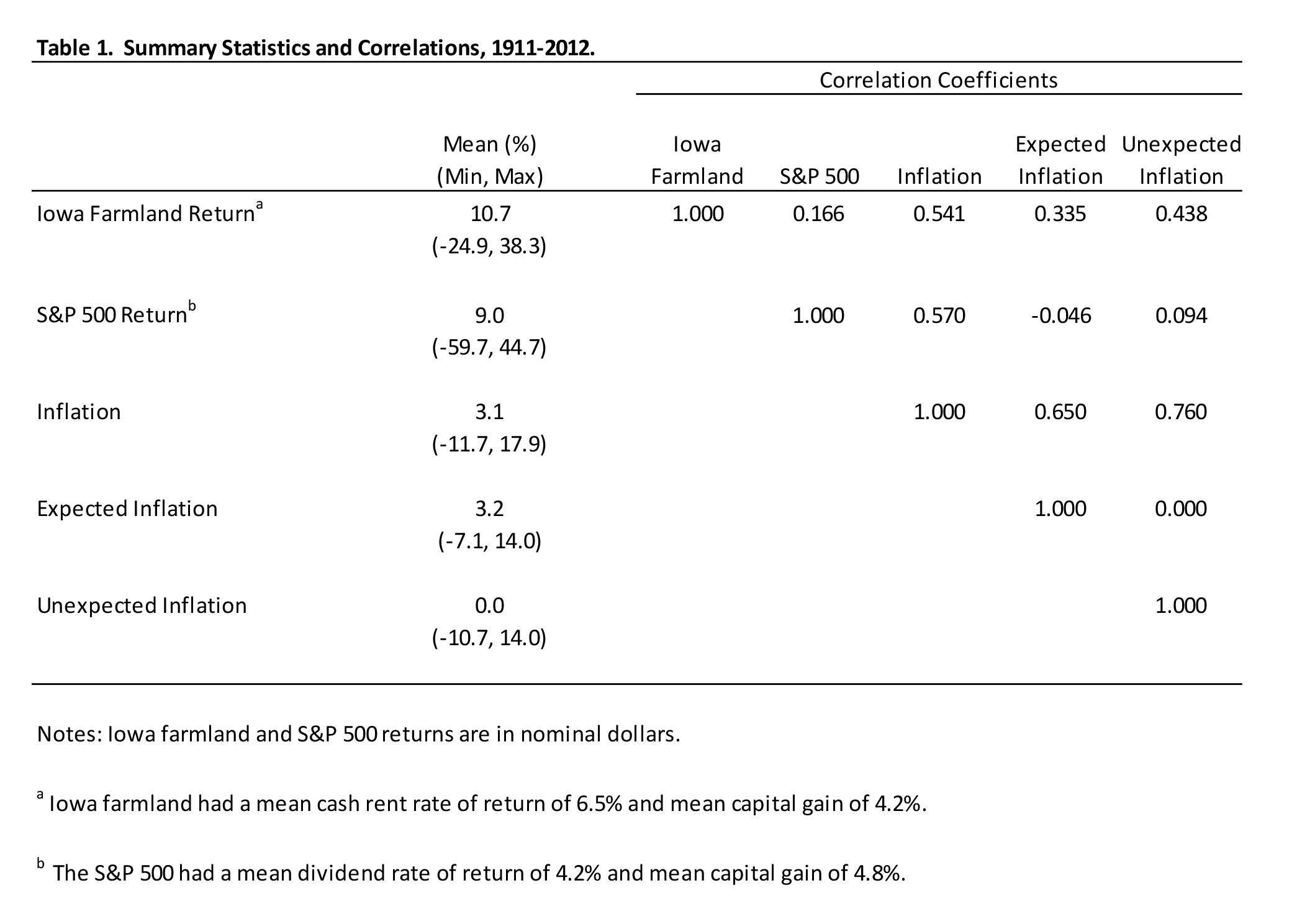
Table 1. Summary Statistics and Correlations, 1911-2012.
Annual returns for the S&P 500 range considerably lower on the negative side (- 59.7%) than Iowa farmland (-24.9%). Inflation ranges from -11.7% to 17.9%, with a mean of 3.1%. Correlations in Table 1 show that farmland has a higher correlation with inflation (.541) than the S&P 500 return (-0.046).
To determine the risk of farmland when added to a well-diversified portfolio, Iowa farmland returns were regressed against S&P 500 returns (Table 2). For comparison purposes, gold and housing price changes were also regressed against S&P 500 returns. The results show a beta of 0.1068 for farmland. Peter Barry published a similar regression in 1980 for U.S. farmland with larger but still relatively low beta of 0.19. Irwin, Forster, and Sherrick (1988) estimated one and two factor models for sample periods 1950-1977 and 1947-1984 and found similar market beta’s to that of Barry, who used the data period 1950-1977, but their market betas are larger for the more recent period (.32 in the one factor model and .25 in the two factor model). In contrast our sample period starts considerably earlier and ends considerably later and we find a beta smaller than Barry’s. However, in the big picture, all of these betas are relatively small, indicating systematic risk much smaller than an average stock. These results support the conventional wisdom that farmland adds little risk to a well-diversified investment portfolio, although the results indicate that gold and housing add even less risk to a well- diversified portfolio with betas of -0.0285 and 0.00025 for gold and housing, respectively.
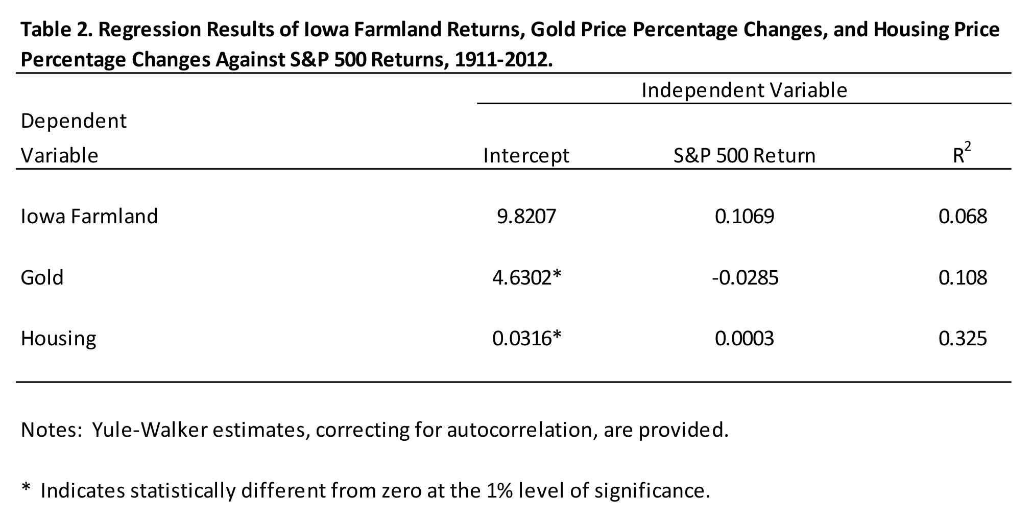
Table 2. Regression Results of Iowa Farmland Returns, Gold Price Percentage Changes, and Housing Price Percentage Changes Against S&P 500 Returns, 1911-2012.
A substantial body of literature following from Fama and Schwert (1977) measures the movement returns for various asset classes with inflation by regressing returns against expected and unexpected inflation. The literature varies in the measures used for expected and unexpected inflation. Fama and Schwert (1977) used short term interest rates as a proxy for expected inflation. We follow Caporale and Jung (1997) and assume that economic agents predict inflation based on past values of inflation. Expected inflation is determined as the predicted value from regressing current inflation on past inflation with two lags6. Unexpected inflation is the residual from that regression.
We compared farmland to stocks as a hedge against inflation. Table 3 summarizes the results of regressing Iowa farmland and S&P 500 returns against expected and unexpected inflation. Results show that Iowa farmland returns move nearly one for one with both expected and unexpected inflation. In contrast, S&P 500 returns move slightly in the opposite direction of expected inflation, and less than half (0.474) times unexpected inflation. The conventional wisdom that farmland is a good hedge against inflation is supported by these results.
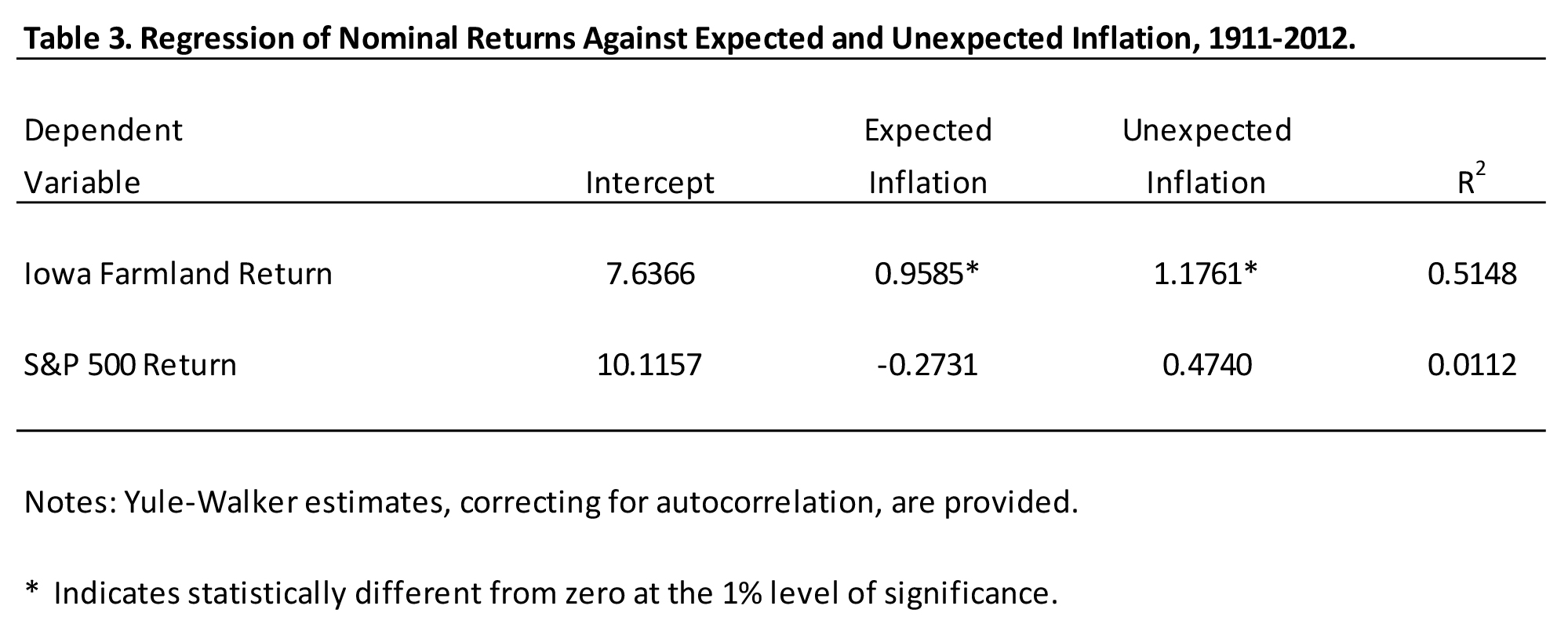
Table 3. Regression of Nominal Returns Against Expected and Unexpected Inflation, 1911-2012.
Conclusions
We have attempted in this paper to provide evidence and insight into the attractiveness of farmland as an investment portfolio choice – – the long-run risk, return, and inflation hedge characteristics of farmland compared to other financial/asset investments. Our analyses use standard financial metrics such as P/E ratios, rates of return, and beta (β) to inform these analyses. The results suggest that the current P/rent ratio for farmland is substantially higher than the historical ratio, and that this ratio is also high relative to the comparable P/E ratio on equities as measured by the S&P 500.
The analysis of historical rates of return for farmland indicates that it has returns comparable to that of stock investments. The risk of farmland as a component of a diversified portfolio as measured by the beta (β) is very low, suggesting it adds little risk to a diversified portfolio. And the inflation hedge results suggest that farmland is a very attractive inflation (both expected and unexpected) hedge investment, much superior to stock investments.
We investigate historical cyclically adjusted P/rent ratios for farmland and find a negative relationship between 10- and 20-year holding returns and the cyclically adjusted P/rent ratio at the time of purchase. Given the extremely high value of farmland P/rent10 in 2013, we suggest caution. Even though our data confirms the conventional wisdom that farmland has high returns, low risk, and is a good inflation hedge, the current P/rent10 ratio suggests this is not a good time to buy. Those purchasing farmland today should not ignore the prospects of “buyer’s remorse”.
References
Bowman, Angela “Is farmland caught in a price bubble that’s about to burst” 2013 [web page] Retrieved from http://www.agprofessional.com/news/Farmland-bubble-faces-moment-of- truth-228809671.html
Burt, O.R. “Econometric Modeling of the Capitalization Formula for Farmland Prices.” American Journal of Agricultural Economics. 68(February 1986): 10-26.
Dobbins, C.L. and K. Cook. “Up Again: Indiana’s Farmland Market in 2013.” Purdue Agricultural Economics Report, August 2013.
Dobbins, C.L., M.R. Langemeier, W.A. Miller, B. Nielsen, T.J. Vyn, S. Casteel, B. Johnson, and K. Wise. “2014 Purdue Crop Cost & Return Guide.” ID-166-W, Purdue University Cooperative Extension, September 2013.
Featherstone, A.M. and T.G. Baker. “An Examination of Farm Sector Real Asset Dynamics: 1910-85.” American Journal of Agricultural Economics. 69(August 1987): 532-546.
Featherstone, A.M. and T.G. Baker. “Effects of Reduced Price and Income Supports on Farmland Rent and Value.” North Central Journal of Agricultural Economics. 10(July 1988):177-189.
Forbes, Steve. Steve Romick: Trade Into the Gold You Can Eat, Farmland. [Web page] (2013) Retrieved from http://www.forbes.com/sites/steveforbes/2013/04/23/steve-romick-trade-into-the-gold-you-can-eat-farmland/
Gustke, Constance. How to invest in farmland [Web page] (2013) Retrieved from http://www.bankrate.com/finance/investing/how-to-invest-in-farmland.aspx
Irwin, Scott H., D. Lynn Forster, and Bruce J. Sherrick. “Returns to farm real estate revisited.” American Journal of Agricultural Economics 70.3 (1988): 580-587.
Lube, Matthew. The Ins and Outs of Farmland Investing [Web page] (2013) Retrieved from http://beta.fool.com/whichstockswork/2013/06/06/the-ins-and-outs-of-farmland-investing/36159/
Moss and Katchova, 2005 “Farmland Valuation and Asset Performance”, Agricultural Finance Review, Volume 65, Issue 2, p-119 to 130.
Robinson, Jerry. Investing in Farmland: 4 Ways to Play the Agricultural Boom. [Web page] (2013) Retrieved from http://www.financialsense.com/contributors/jerry-robinson/investing-farmland-four-ways-play-agricultural-boom
Shiller, R.J. Irrational Exuberance, 2nd Edition. New York: Crown Business, 2005. Shiller, R.J. Irrational Exuberance, 2nd Edition. Web Site: www.irrationalexuberance.com,
accessed on September 18, 2013.
Watts. William L. “Farmland Bubble? 10-year rise raises red flags” 2013 [web site] Retrieved
from http://www.marketwatch.com/story/farmland-bubble-10-year-rise-raises-red-flags-2013-10-21
![]()
![]()
![]()
![]()
![]()
TAGS:
TEAM LINKS:
RELATED RESOURCES
UPCOMING EVENTS
We are taking a short break, but please plan to join us at one of our future programs that is a little farther in the future.