March 28, 2013
Farmland Price to Earnings Ratios for Indiana
![]()
![]()
![]()
![]()
![]()
Abstract
This paper explores trends in farmland values, cash rents, interest rates, the farmland price to cash rent (P/Rent) multiple, and the price to earnings (P/E) ratio on stocks. The P/Rent multiple averaged 17.6 from 1960 to 2012 and ranged from 11.1 in 1986 to 29.5 in 2012. Comparisons of the P/Rent ratio to the P/E ratio indicated that the current P/Rent ratio is above the current P/E ratio and substantially above both the long-term P/Rent and P/E ratios. A negative relationship between the P/rent ratio at the time of purchase and 10-year and 20-year rates of return for holding land was found. The results presented in this paper should make those considering purchasing land at current prices cautious.
Introduction
Farmland values have been rising rapidly in recent years. There is concern by many that farmland prices will become higher than justified by the fundamentals and result in what we will later recognize as a bubble. One justification for this concern is that previous research has established the tendency of the farmland market to over shoot (Burt, 1986; Featherstone and Baker, 1987; Featherstone and Baker, 1988). So, from the standpoint of the literature and history, another bubble in farmland prices would not be a surprise.
This paper explores trends in farmland price, cash rents, interest rates, the farmland price to cash rent multiple, and the price to earnings ratios for stocks. Emphasis will be placed on the similarities and differences between the farmland price to cash rent multiple (P/Rent) and the price-earnings (P/E) ratio of the S&P 500 stock index, a metric commonly used in the financial markets to assess the relationship between the price of stock and the earnings generated by the company. The premise is that earnings are a fundamental determinant of the value of an asset or investment, and that an abnormally high P/E ratio suggests that forces other than current earnings are influencing values or asset prices, presenting the prospects of overvaluation based on fundamentals.
The Analytical Framework
The present value model noted above is directly related to the income approach to valuation used in appraisal which divides the return to land by a capitalization rate:
If the cash rental rate is used as the return to land, then the reciprocal of the cap rate is the P/rent multiple, the focus in this paper.
The constant growth present value model is often used as the theory behind the income capitalization model. This model allows us to examine the fundamental factors determining farmland value. In this model, the return to an asset at the current time (R0) is expected to grow at rate g indefinitely, and the required rate of return is r, leading to the following present value model.
Solution to the infinite series of equation (2) yields the constant growth model (3):
In equation (3), the capitalization rate is the difference between the required rate of return (r) and the anticipated indefinite constant growth rate (g). The P/rent multiple will increase as the difference r-g declines, which means that reducing the required rate of return, or increasing the expected long-term growth in rent are the two factors that will increase the multiple. It is difficult to determine how the land market views these two factors. Empirical econometric work from the 1980s found little to no effect of changing interest rates on land values, which supported the constant capitalization rate hypothesis (Burt, 1986; Featherstone and Baker, 1987; Featherstone and Baker, 1988). Since the required rate of return and growth rate are long-run constant values in the model, it is perhaps logical to think that these values would be slow to change in response to current conditions. At the same time, sustained experience of high growth in cash rent or experience of sustained periods with low interest rates (both of which have been the case for the past decade or so) might influence investor’s expectations of these factors and thus increase the multiple.
The fundamentals of land price increases can be seen from the constant growth model. Land prices increase either because returns to land increase or because the multiple increases. The multiple increases when the required return, r, decreases relative to the expected long-run growth rate, g. In this paper we use cash rent as our measure of return to land. It is very possible that at a given point in time the level of rent and the multiple are not independent factors. Most of our discussion will treat the two factors separately, but, for example, at a given time average rent reported in surveys could be a clear notch or two lower than the market expects in the near future and the result would be the appearance of an abnormally high multiple.
P/E ratios for stocks are compared to the price to earnings multiple (P/rent) for farmland in this paper. The P/E ratio is computed by dividing market value per share for a particular stock or group of stocks to the appropriate earnings per share (EPS). Historical or expected earnings per share can be used in the computation. P/E ratios reported typically use historical earnings per share to compute the ratio. The average market P/E ratio for stocks is 15 to 20 however, it is important to note that the average P/E ratio does vary across industries. In general, a high P/E ratio indicates that investors anticipate higher growth of earnings in the future.
Data
Some of the main sources of farmland price data are surveys by Universities, Federal Reserve Banks, and USDA. In this paper we draw on a cash rent and farmland price series for West Central Indiana from the annual Purdue survey of Indiana farmland values from 1974 to 2012. The most recent survey is reported in Dobbins and Cook (2012). We have extended the 1974 to 2012 Purdue survey data back to 1960 using USDA data. One of the characteristics of survey data is that it tends to average out the highest farmland prices one hears about (i.e., anecdotal prices). Survey cash rent numbers also are lower than the highest prices that we know that some landowners are receiving. So, during the time that the farmland market is moving up, survey prices and cash rents often lag behind what is actually happening. We will present figures and tables using historical survey data. There are not strong arguments that the current survey data reflect a bubble in the farmland market. What we are more worried about are the indications from reports of sales from anecdotal sources that farmland prices have moved up well beyond the survey reports.
The reason for using West Central Indiana farmland prices and cash rent is because we have budgeted “actual” owner operator returns using actual yields from one of the counties in the West Central region. We use Tippecanoe County county average yields of corn and soybeans, season average prices of corn and soybeans, costs primarily from Purdue Crop Budgets (e.g., Dobbins et al., 2012), Environmental Working Group data for government payments for the years available (budgeted government payments for earlier years), and a 50-50 corn-soybean rotation to compute historical owner operator returns. These returns are the most important factor driving the cash rental market which is our best indicator of the return to land (albeit a measure of return before landlord costs such as property taxes are subtracted).
We also compare stock P/E ratios to the farmland price to earnings ratio (P/rent) in this paper. The P/E ratio data for individual stocks is obtained from Yahoo Finance (www.finance.yahoo.com). The S&P data was obtained from various web sites and Shiller.
P/Rent and Interest Rates
Farmland prices, cash rents, and owner operator returns for West Central Indiana are shown in figure 1. The figure is in current prices or nominal dollars. Land prices are represented on the left axis while cash rents and owner operator returns are represented on the right axis. In nominal dollars, the bubble in the 70s and 80s is barely noticeable. It is noticeable in figure 1 that land prices since the mid-1990s have risen more than cash rents. This results in a strong upward trend in the price-to-cash-rent-multiple (P/rent) shown in figure 2.
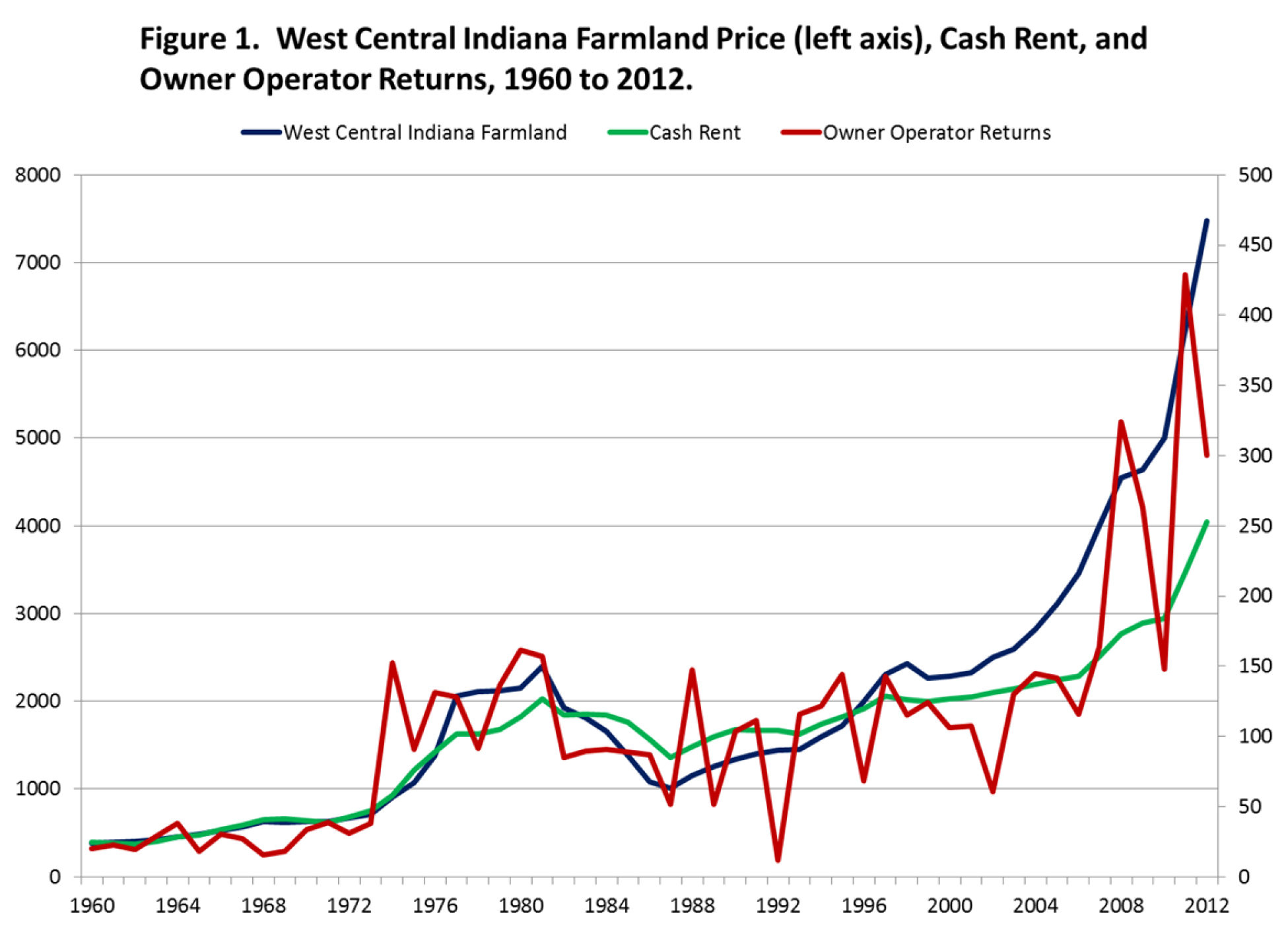
Figure 1. West Central Indiana Farmland Price, Cash Rent, and Owner Operator Returns, 1960 to 2012.
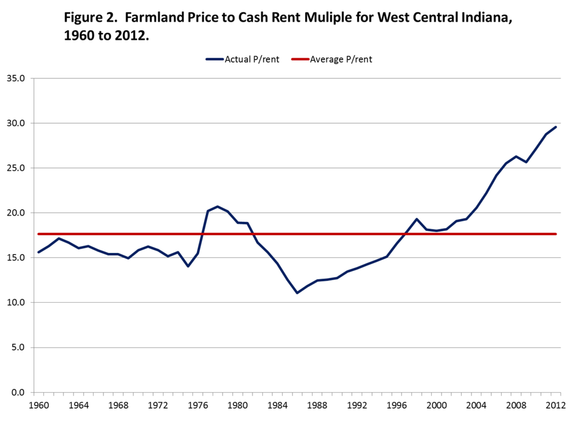
Figure 2. Farmland Price to Cash Rent Multiple for West Central Indiana, 1960 to 2012.
The P/rent ratio for West Central Indiana has an average value of 17.6 over the 52 year period with a high of 29.5 reached in the last year of data (2012) and a low of 11.1 in 1986, which was perhaps the bottom of the valley after the bubble of the 1970s and 1980s. At the peak of this bubble, the P/Rent multiple reached a high of just over 20 from 1977 through 1979. The P/Rent multiple subsequently dropped to the teens in the early 1980s, and down to its low in 1986. The rise from around 15 in 1976 into the 20s and down to 11.1 in 1986 corresponds exactly to what is viewed as the bubble in land prices and one of the more difficult periods for agriculture in modern history. It is within this historical context that the rise in the P/rent ratio to the upper teens in the later 1990s and then well above 20 in the 2000s, climbing higher and higher through the last survey value of 29.5 is of alarm.
Examining the behavior of the P/rent multiple in the 1970s and 1980s (figure 2), we see that the multiple increased from about 15 to about 20, and this increase was a key part of what we think of as the bubble in land prices at that time. It is hard to rationalize the increase being due to interest rates, because nominal interest rates became very high at that time. But inflation was also high in this period, and during part of the period real interest rates (i.e., inflation adjusted interest rates) were low, so maybe low real rates of interest are a partial explanation for the increasing P/rent multiple during this period.
Another possible explanation is that the high growth rate in cash rent in the 1970s created expectations of higher long-run growth in cash rent. The average growth rate in cash rent from 1960 through 2012 is 4.5%, but from 1972 through 1977, cash rent grew at an average rate of 16.2% with a minimum of 9.4% in 1972 and a maximum of 27.0% in 1975. Basing expectations of future growth on recent growth would result in an expectations process that would increase the chances of cyclical bubbles. A counterbalancing expectations mechanism might be one in which high growth rates lead to decreased expectations of future growth. In other words, when cash rent increases a large percentage over several years, the market participants might say “cash rent has gotten very high, times are good, and this rate of improvement can’t last”, rather than implicitly saying by paying a high P/rent multiple for farmland that “cash rent has really gone up, I’ll bet this high rate of improvement is going to last forever.”
This leads us to the period from the 1990s to today and the growing and historically high farmland P/rent ratio (figure 2). Ten-year US Treasury average annual interest rates have fallen fairly steadily from a peak of 13.1% in 1981 to 1.8% in 2012 (figure 3). The required rate of return by farmland investors would be higher than the 10-year U.S. Treasury interest rate due to a risk premium, which one might expect to be at least as large as the premium of the farm borrowing rate over the 10-year U.S. Treasury rate which is 1.99%1. If farmland market participants have required rates of return for farmland that follow the 10-year Treasury rate (plus a constant risk premium), then the time series pattern shown by the 10-year Treasury rate would give us an indication of the direction of change in the discount rate in the constant growth model. If the risk premium and expected growth rate approximately canceled each other, then the reciprocal of the 10-year Treasury rate would approximate the price to rent multiple.
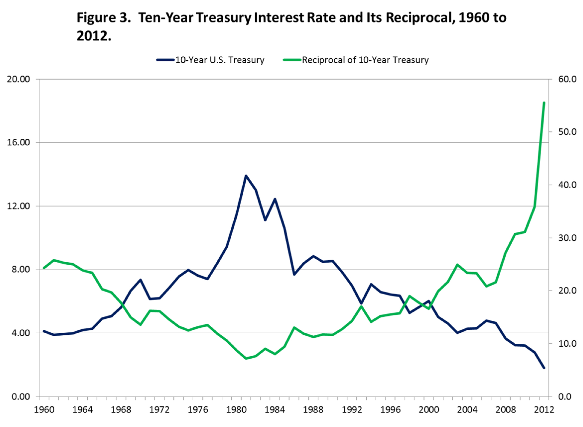
Figure 3. Ten-Year Treasury Interest Rate and Its Reciprocal, 1960 to 2012.
The reciprocal of the 10-year Treasury interest rate tracks the increase in the farmland P/rent ratio quite well from 1985 to 2010 (figure 4). In the period from 1960 to 1985 there is not an obvious connection between the P/rent ratio and the 10-year Treasury interest rate. Also, the relationship has diverged during the last several years. If the recent very high P/Rent ratios are caused by the recent extremely low interest rates (which results in a high reciprocal), then the implication is that the market expects these low rates to continue over the long term. This again is a troubling factor with respect to the ability of the current high land prices to be sustained. Interest rate futures markets and a positive slope in the Treasury yield curve have been predicting rising interest rates for the last two years, and even though this has not occurred, it is reasonable to question the long-run persistence of the perpetually low interest rates that would be required as the fundamental to justify high P/rent ratios.
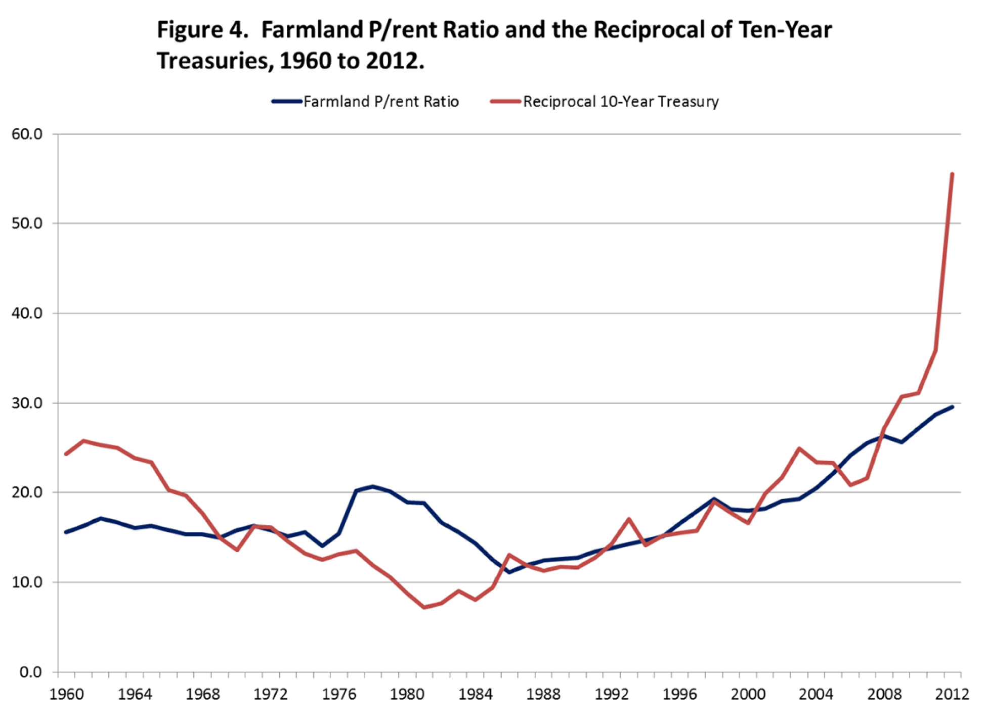
Figure 4. Farmland P/rent Ratio and the Reciprocal of Ten-Year Treasuries, 1960 to 2012.
Similarities Between P/Rent and P/E Ratios
The P/E ratio shows the price one must pay when buying shares of stock to purchase $1 of a company’s current earnings, which is similar to the P/Rent ratio which shows the price paid to purchase enough land to buy $1 of current returns to land. Cash rent for one acre of land for the 2012 was $253 (Table 1) and that acre of land was worth $7,475. The cost of purchasing $253 of current earnings is significantly lower than the cost of an acre of farmland for Tyson ($3,670), Hormel ($5,241), Deere ($2,892), and Caterpillar ($2,720). The dollar amounts above represent the P/E ratios multiplied by 253, the current cash rent for West Central Indiana.
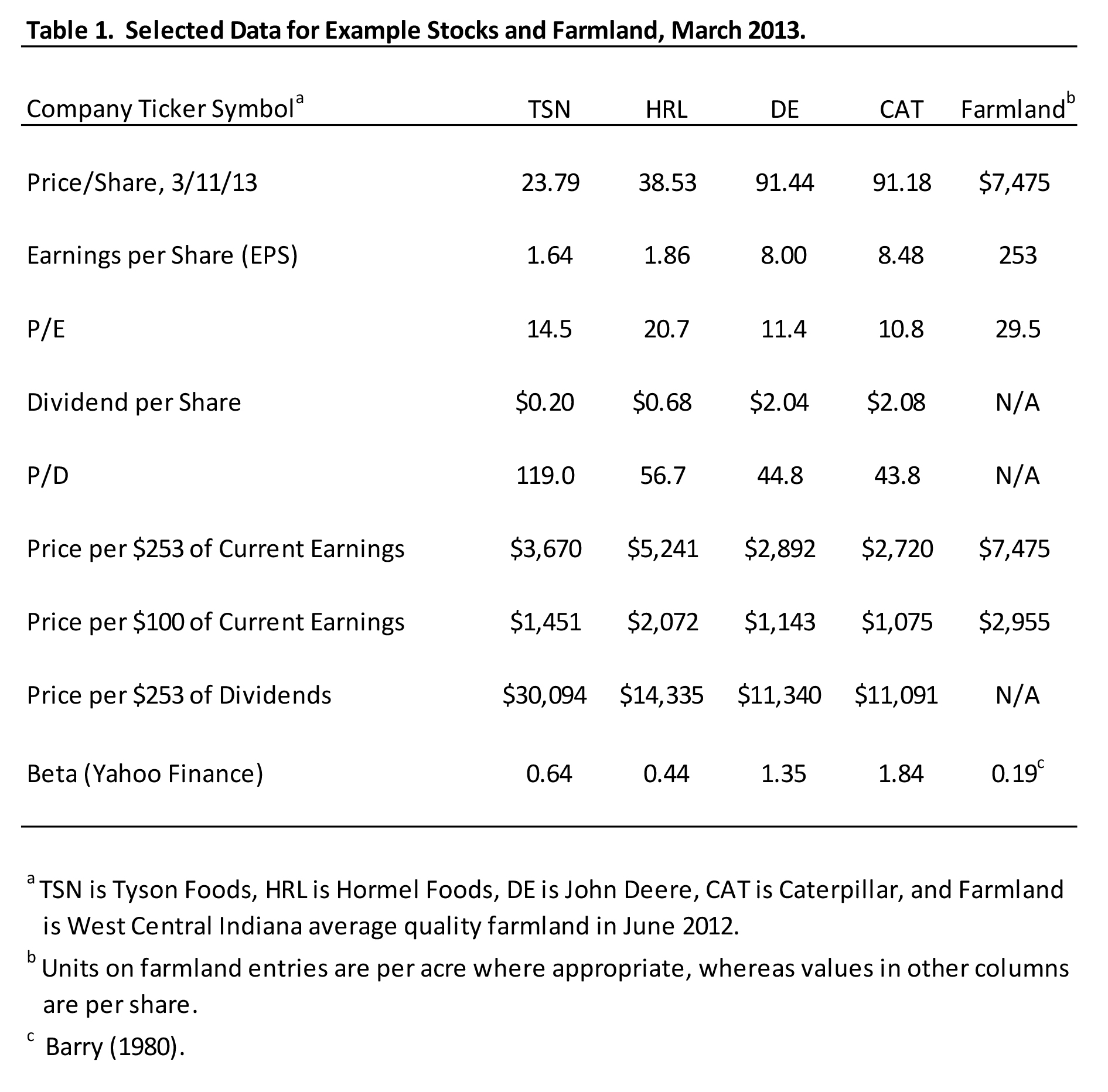
Table 1. Selected Data for Example Stocks and Farmland, March 2013.
The primary reason one would pay more for a dollar of current earnings for one company or asset over another is that you expect future earnings to grow more rapidly for that company. Farmland is priced at about 42% above the earnings multiple for Hormel, and more than double that for agribusinesses Tyson, Deere, and Caterpillar. One might want to contemplate why the future prospects of growth in earnings are perceived to be so much better for farmland than for agribusiness stocks.
The second reason one would pay a different price per dollar of current earnings is risk. If risk is higher, then the discount rate for future earnings will be higher. So, even if future earnings are the same for two assets, the one with higher risk would have a higher required rate of return and therefore a lower value. Beta is a measure of how the rate of return on investing in an asset moves with the return on the whole market (Brealey, Myers, and Allen, 2013). Beta measures the contribution of an asset to the risk of a well-diversified portfolio. Farmland has been estimated to have a very low beta (table 1), but it is not entirely clear that the measure is appropriate as investors in farmland do not perhaps have a well-diversified portfolios.
The P/rent ratio can also be compared to stock market indices. Figure 5 shows the P/E ratio for the S&P 500 and the P/rent ratio. The average P/E ratio for the S&P 500 for the period at 18.1 is fairly close to the 17.6 average for the P/rent ratio for farmland. The S&P 500 P/E ratio and the P/Rent ratio for land are positively correlated over the period at 0.215 (table 2). In most of the years since 1985 the P/E ratio has been higher than the P/Rent ratio. However, the 2011 and 2012 P/rent ratios are higher than the corresponding P/E ratios, which is disconcerting. Also, the P/rent ratio has exhibited an upward trend. The current P/Rent ratio of 29.5 is well above the average P/E multiple. Variation in the P/E ratio is the result of variations in earnings. At times earnings are low, but are not expected to remain low, so the P/E ratio shoots up. This type of effect is not as large of a factor in the farmland market.
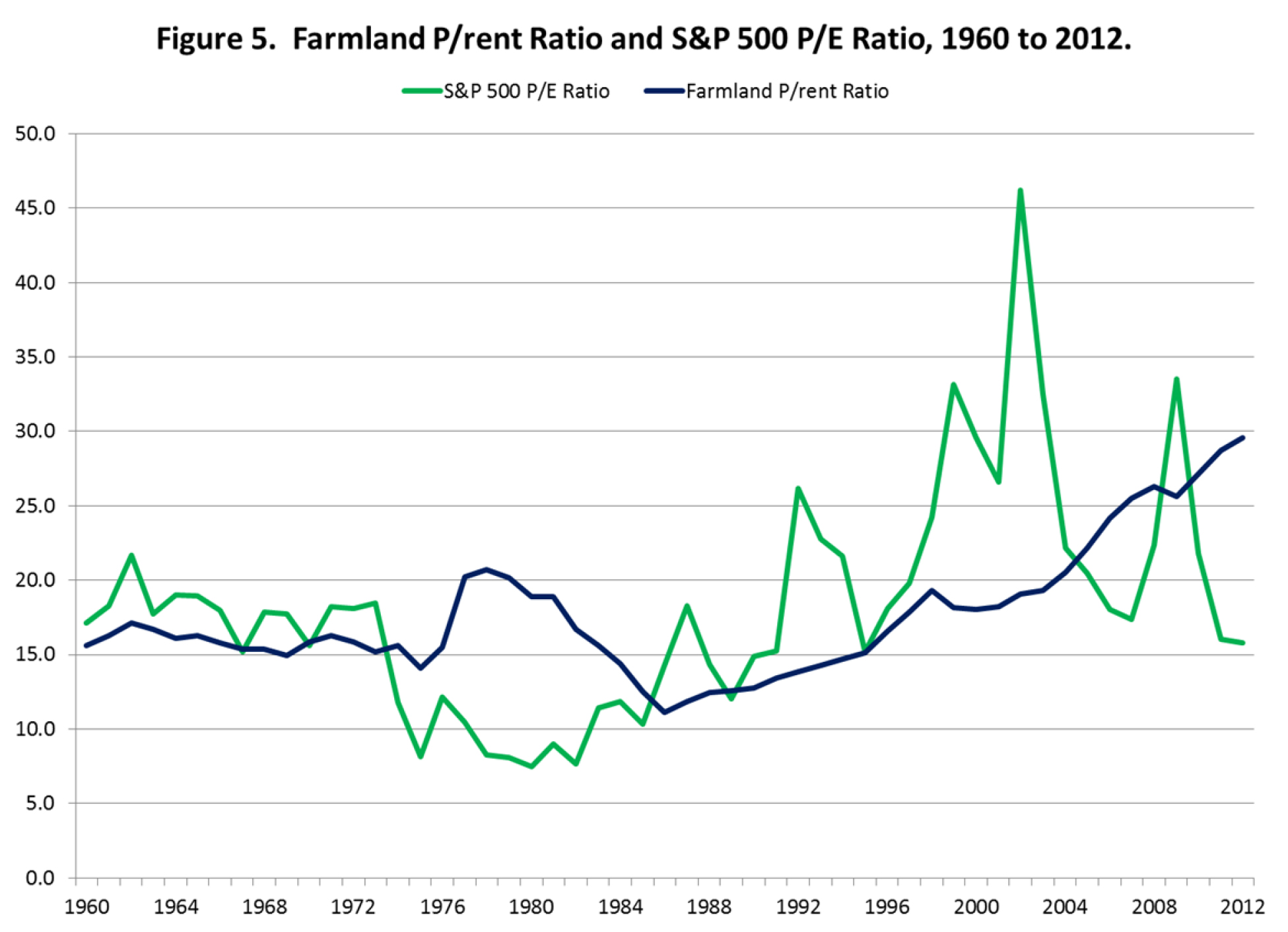
Figure 5. Farmland P/rent Ratio and S&P 500 P/E Ratio, 1960 to 2012.
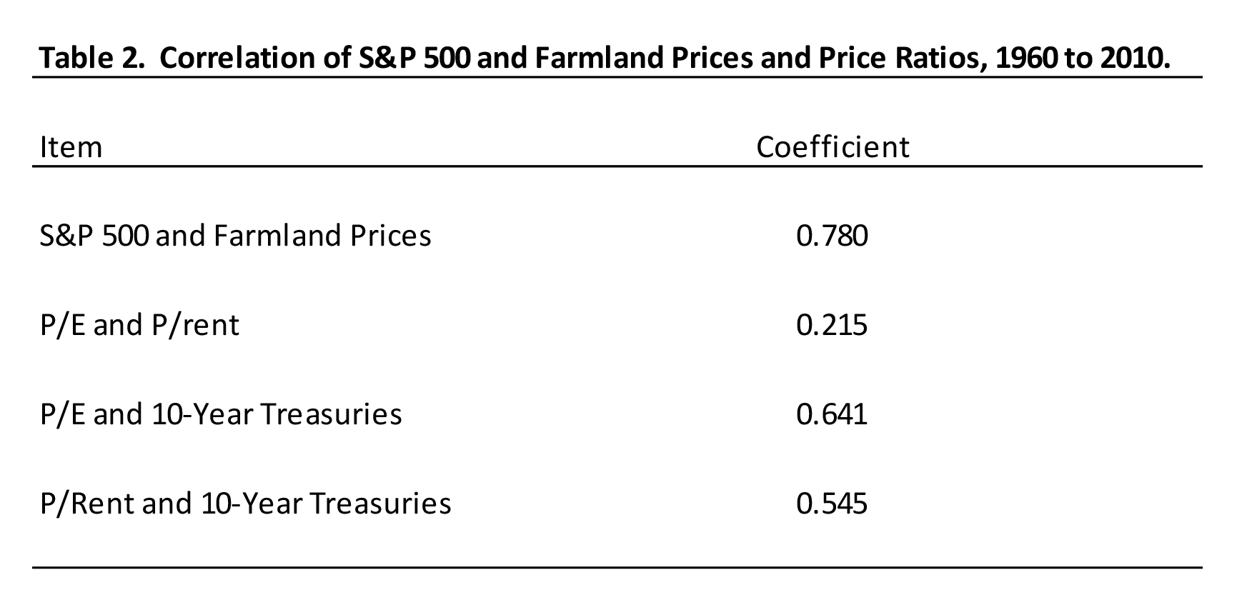
Table 2. Correlation of S&P 500 and Farmland Prices and Price Ratios, 1960 to 2010.
There are shortcomings to comparing P/rent and P/E ratios. Cash flow received by a stock investor is the dividend on the stock, not the earnings. The percentage of earnings per share (EPS) paid out as dividends vary from company to company, ranging from zero to over 100 percent. Historically, the dividend payment ratio for the S&P 500 has averaged about 55%. In recent years, this ratio has been closer to 30%. If part of earnings is retained, then equity is increased and future earnings should be greater because there would be earnings on the larger equity base. This is a continual process and one of the fundamental reasons why one would expect growth in earnings of a corporation.2 Innovations from research and development; inflation; efficiency improvements; increased demand due to income, population, and advertising; and other reasons would also be behind growth in income of corporations. Growth in returns to farmland would have a similar list of drivers, except there is not a factor for farmland comparable to a corporation’s retaining earnings to increase the firm’s equity base. However, over time the value of a corporation’s patents and intellectual property, barriers to entry, and market power may erode, which would diminish growth in earnings or even cause earnings to decline.
Dividends are of course smaller than earnings, so Price/Dividend (P/D) ratios are higher than P/E ratios. The prices of shares of stock in companies reflect both the dividend payout and the effect of retention on expected growth. The effect of changing payout and retention rates is masked when looking at the P/E ratio at different times and comparing different companies. If one owns an acre of farmland and rents it for $253 the cash flow received is $253 (less landlord expenses which we ignore here). In table 1 we see that the price paid for $253 of cash flow (dividends) is much higher for the agribusinesses; ranging from $11,091 for Caterpillar to $30,094 for Tyson; than for an acre of land ($7,475). However, it should be noted that comparing P/D ratios of individual companies to farmland is probably of limited value because of the extreme variation in the situation for each company.
Growth in Farmland Returns
As previously indicated, the expected long-run future growth rate in farmland returns is one of the key variables in the constant growth model and is a major determinate of the P/rent ratio. In the constant growth model, the variable g is constant over an infinite horizon. While constant growth over an infinite horizon is clearly an approximation of reality, in this section we are thinking about growth in returns as a long-run concept.
Farmland market participants likely look at past growth in rent when anticipating future growth because it is human nature to use past experience when assessing the future. Thus, one would expect participants in the farmland market to be looking at past growth in returns along with current information about drivers of that growth to base their expectations.
Growth in cash rent (year-over-year continuous percentage change)3 and the 5-year moving average growth rate is shown in figure 6. Extremely high growth rates in cash rent were experienced in the middle 1970s. The growth rates of course fell through the middle 1980s. The 5-year moving average smooths the year to year changes in annual growth and lags substantial increases and decreases in growth, but generally speaking followed the same pattern. In economic models moving averages are sometimes used to model or represent market participant expectations. While the 5-year moving average might be a good indicator of the optimism or pessimism of those in agriculture, it is hard to believe that farmland market participants expected long-term growth in the -5% range in the later 1980s, but surely the anticipated growth in the 1980s was lower than what it was in the mid-1970s. If market participants did have expectations following a moving average it would explain the markets tendency to over and under shoot. If recent growth in rent has been high, the moving average increases and if the expectation of higher growth rate in rent follows, then the P/rent ratio would increase. The reverse would happen when rents fall. Thus, land values would be increasing or decreasing both because rents increase or decrease and because the P/rent multiple increases or decreases.
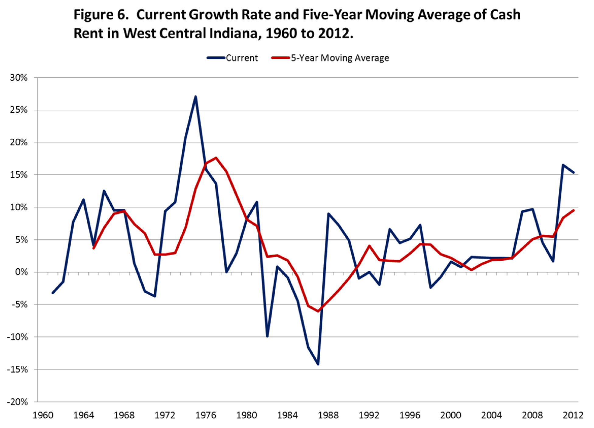
Figure 6. Current Growth Rate and Five-Year Moving Average of Cash Rent in West Central Indiana, 1960 to 2012.
The mean growth in returns to land over the last 50 years has been 4.5%. The 5-year and 10-year moving averages of growth rates in cash rent have movements that are similar to the patterns shown in the farmland P/rent ratio (figure 7).
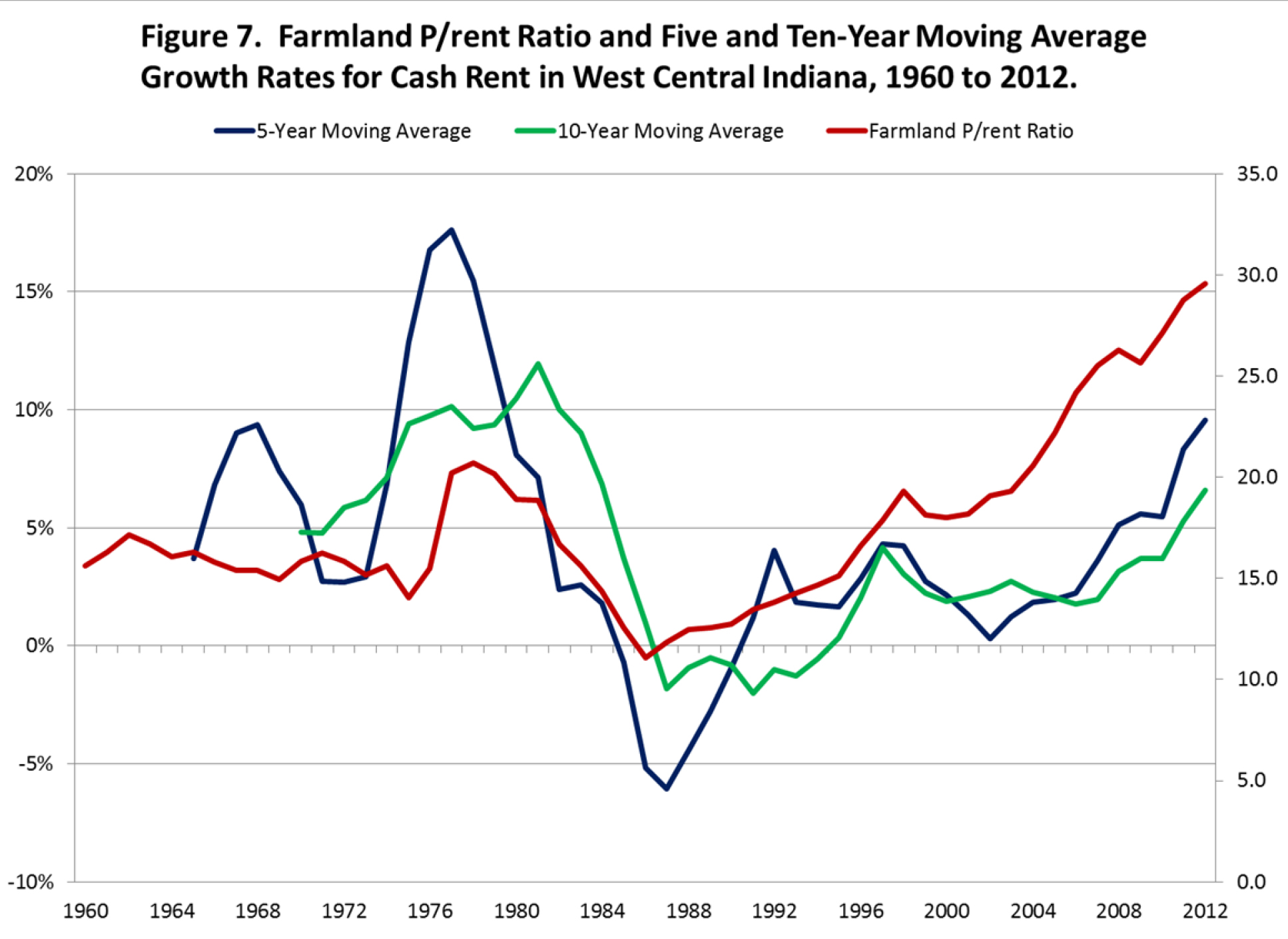
Figure 7. Farmland P/rent Ratio and Five and Ten-Year Moving Average Growth Rates for Cash Rent in West Central Indiana, 1960 to 2012.
Cyclically Adjusted P/rent
Shiller (2005; 2013) uses a 10-year moving average for earnings (often labeled either P/E10 or CAPE) in order to remove the effect of the economic cycle on the P/E ratio. CAPE is an acronym for cyclically adjusted P/E. When earnings collapse in recessions stock prices often do not fall as much as earnings and the P/E ratios based on the low current earnings sometimes become very large. Similarly, in good economic times P/E ratios can fall and stocks look cheap, simply because the very high current earnings are not expected to last, so stock prices do not go up by as much as earnings. By using a 10-year average of earnings in the denominator of the P/E ratio, Shiller has smoothed out the business cycle. In Shiller’s calculations he also deflated both earnings and prices to remove the effects of inflation over fairly long period over which is averaging earnings.
In this paper, the P/rent ratio is the current year’s farmland price for West Central Indiana divided by cash rent for the same year. P/rent5 and P/rent10 are modeled after Shiller’s cyclically adjusted P/E ratio. Cash rent and farmland prices are deflated, and then 5 and 10-year moving averages of real cash rent are calculated. P/rent5 is computed by dividing the real farmland price by the 5-year moving average real cash rent. Similarly, the P/rent10 ratio is computed by dividing the real farmland price by the 10-year moving average real cash rent.
In figure 8, current, 5-year, and 10-year rents are used to compute P/rent ratios over the study period. All three P/rent ratios follow an almost identical pattern. The results from dividing land price by the real 5-year moving cash rent and owner operator returns (computed using season average prices, costs from Purdue crop budgets, and yields from Tippecanoe County) are illustrated in figure 9. The opposite pattern is exhibited during rapid increases and decreases in the ratios. The P/OO-5 ratio is above the P/rent5 ratio until 1974. From 1974 to 1990, the P/OO-5 ratio is very stable compared to the P/rent5 ratio which more closely follows the farmland price pattern. From 1985 to 2008 the P/OO-5 ratio is above the P/rent5 ratio, but from 2008 through 2012 the P/rent5 ratio rises, while the P/OO-5 falls and stabilizes.
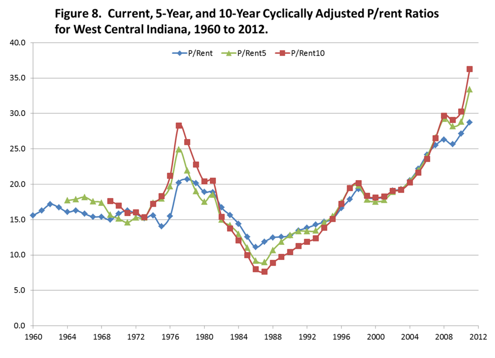
Figure 8. Current, 5-Year, and 10-Year Cyclically Adjusted P/rent Ratios for West Central Indiana, 1960 to 2012.
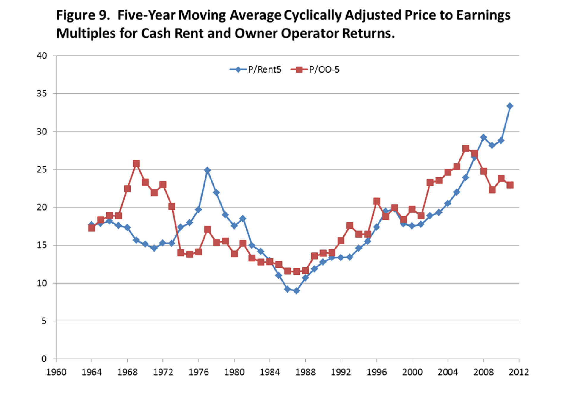
Figure 9. Five-Year Moving Average Cyclically Adjusted Price to Earnings Multiples for Cash Rent and Owner Operator Returns.
In figure 10, we show real land prices divided by 10-year moving average real cash rents and real owner operator returns as well as Shiller’s P/E10 ratio. The 10-year ratios for cash rents and owner operator returns are more comparable to Shiller’s analysis. The P/OO-10 (red line in the graph) fell through the first half of the 1970s when real returns grew faster than land values, increased from the high teens in the middle 1970s to 25.4 in 1977, and then fell to 7.7 in 1986. The P/OO-10 then increased steadily until it reached 32.3 in 2012. For the last couple years, the P/rent10 ratio has been substantially above the P/OO-10 ratio. Two points are evident from figure 10. First, the P/rent ratio is approaching the peak of the P/E ratio during the dot.com bubble. Second, the relationship between the P/rent ratio and the P/OO-10 ratio suggests that producers are not bidding all of the owner operator returns into cash rents. In other words, producers may be expecting owner operator returns to decline, which would make it difficult to maintain high cash rents. However, this relationship could also be explained if one expects cash rents to adjust slowly to changes in operator returns. Historically, there have been times when cash rents were slow to adjust. These phenomena would also explain the recent relationship between the P/rent and P/OO-10 ratios.
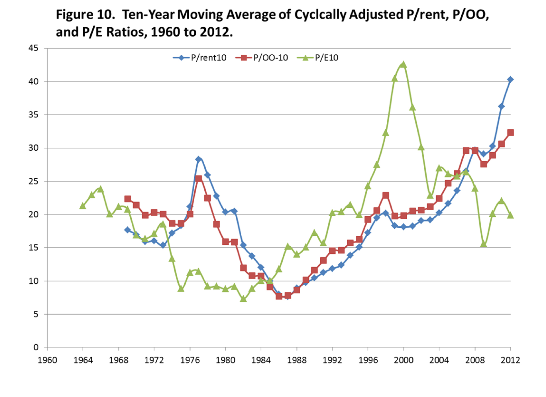
Figure 10. Ten-Year Moving Average of Cyclically Adjusted P/rent, P/OO, and P/E Ratios, 1960 to 2012.
Shiller (2005; 2013) shows the annualized rate of return from holding the S&P 500 for long holding periods. In general, the higher the P/E ratio at the time of purchase, the lower the resulting 10-year returns. Given that we know the historical P/E ratio has gone up or down, the negative relationship is almost a mathematical identity. The farmland and cash rent data from 1960 to 2012 can be used to compute 10-year and 20-year annualized rates of return, which are taken to be the sum of the average of cash rent as a fraction of the farmland price each year plus the annualized price appreciation over the holding period. The results for farmland show the same kind of negative relationship seen in stock data. The 10-year holding period returns for farmland show a strong negative relationship, the higher the P/rent10 (farmland price divided by 10-year moving average of cash rent) at the time of purchase the lower the resulting 10-year rate of return (figure 11). The 10-year holding returns range from a slightly negative rate of return to 20%. The 20-year holding period returns also exhibit a strong negative relationship with the P/rent10 ratio (figure 12). The 20-year holding returns range from 6 to 14%.
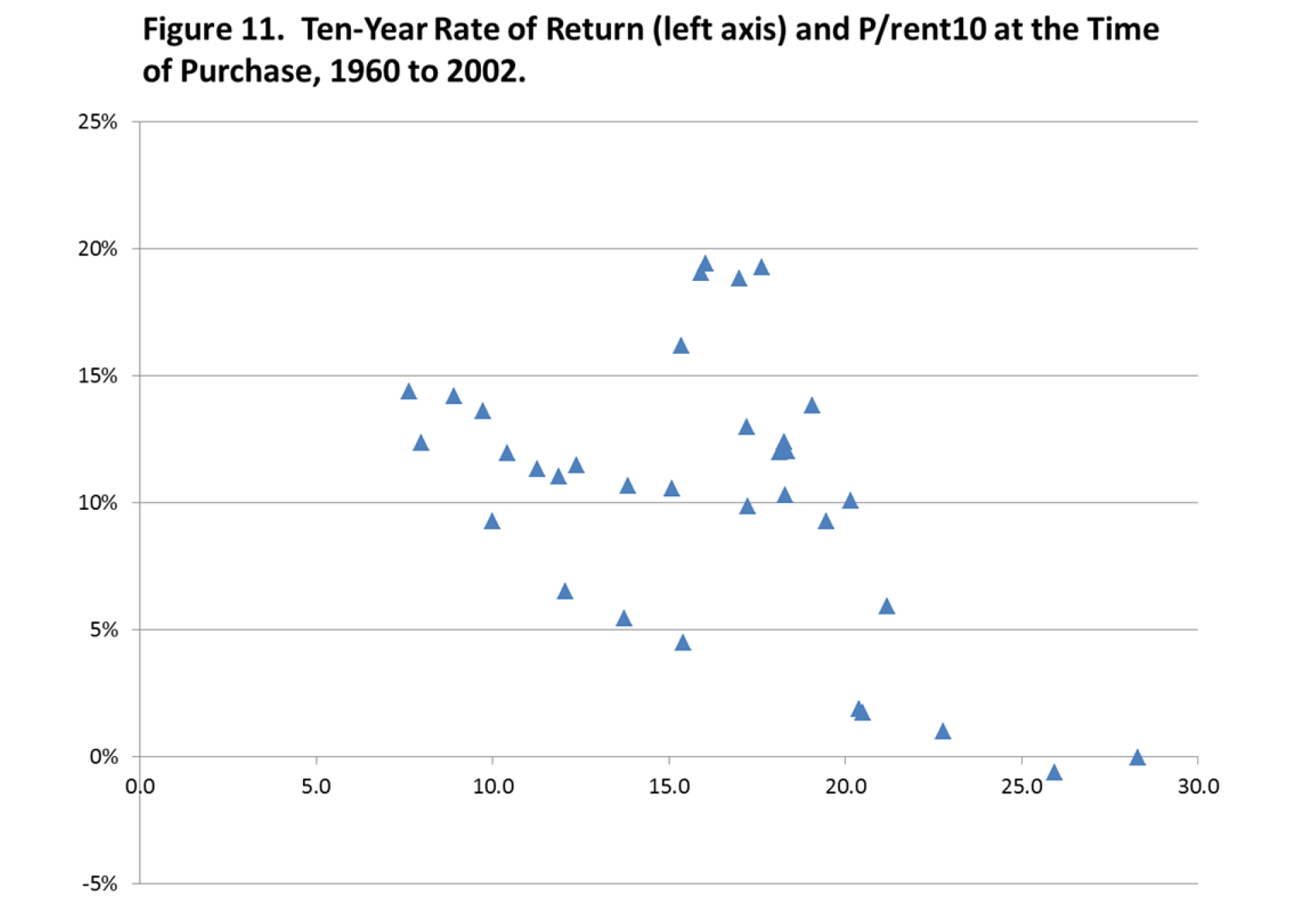
Figure 11. Ten-Year Rate of Return and P/rent10 at the Time of Purchase, 1960 to 2002.
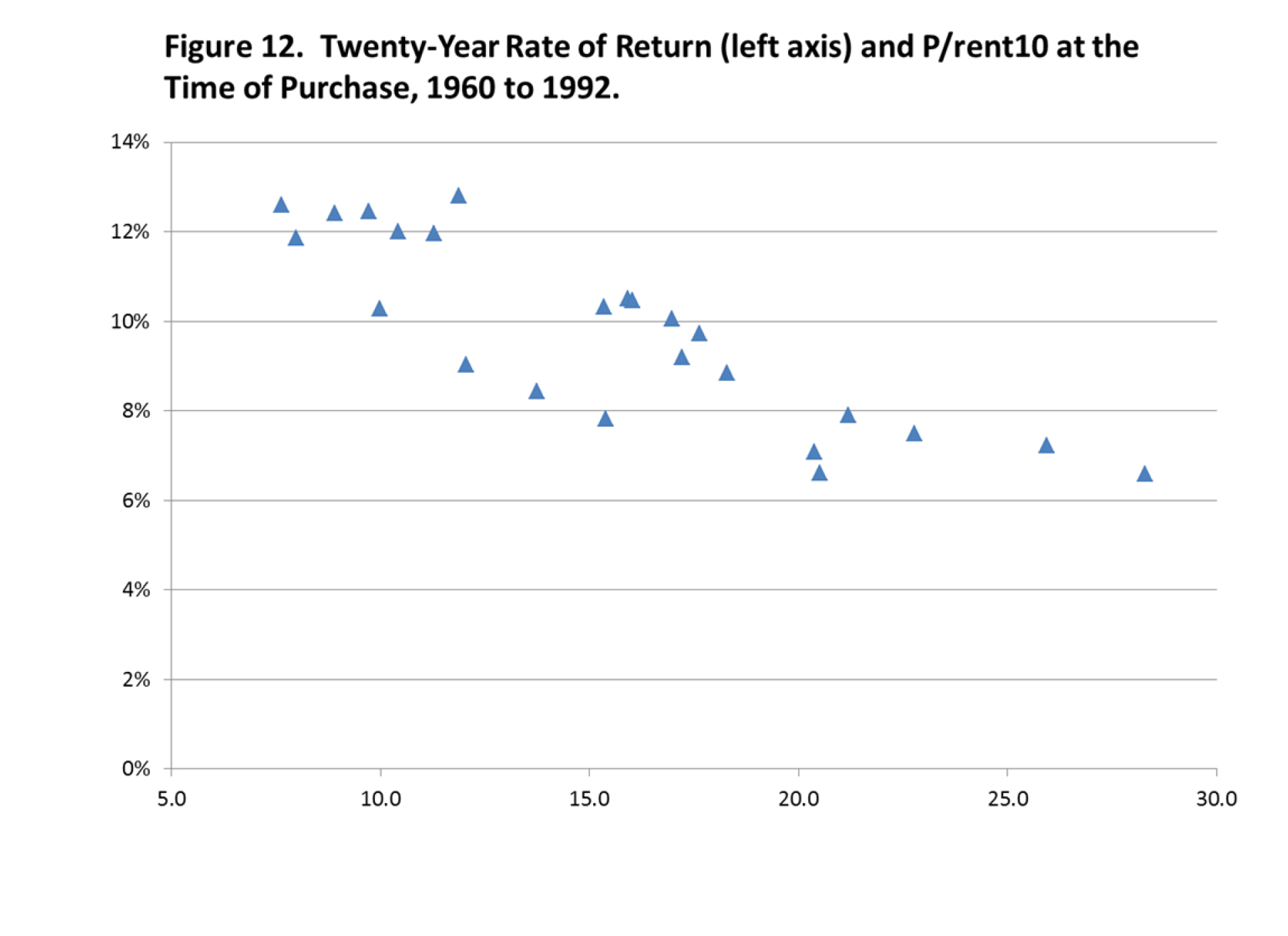
Figure 12. Twenty-Year Rate of Return and P/rent10 at the Time of Purchase, 1960 to 1992.
Summary and Conclusions
This paper examined trends in stock P/E ratios and farmland’s price to cash rent ratios (P/rent). The current P/rent ratio is substantially higher than the historical average P/rent ratio. The P/rent ratio represents the reciprocal of the capitalization rate. The reciprocal of the 10-year Treasury interest rate tracks the increase in the farmland P/rent, thus the rising P/rent ratio may not be as irrational as it seems. However, if the recent very high P/rent ratios are caused by the extremely low interest rates, then the implication is that the market expects these low rates to continue over the long-run, which certainly may not the case.
The cyclically adjusted P/rent ratio was also relatively high. There is typically an inverse relationship between the cyclically adjusted P/rent and P/E ratios and investment returns. This relationship was confirmed in this paper. Those purchasing farmland today or thinking about purchasing farmland in the near future should take this negative relationship into account when bidding on farmland.
References
Barry, P.J. “Capital Asset Pricing and Farm Real Estate.” American Journal of Agricultural Economics. 62(August 1980):549-553.
Brealey, R., S. Myers, and F. Allen. Principles of Corporate Finance, 11th Edition. New York: McGraw-Hill, 2013.
Burt, O.R. “Econometric Modeling of the Capitalization Formula for Farmland Prices.” American Journal of Agricultural Economics. 68(February 1986):10-26.
Dobbins, C.L. and K. Cook. “Indiana’s Farmland Market Continues Moving Higher.” Purdue Agricultural Economics Report, August 2012.
Dobbins, C.L., M.R. Langemeier, W.A. Miller, B. Nielsen, T.J. Vyn, S. Casteel, B. Johnson, and K. Wise. “2013 Purdue Crop Cost & Return Guide.” ID-166-W, Purdue University Cooperative Extension, November 2012.
Featherstone, A.M. and T.G. Baker. “An Examination of Farm Sector Real Asset Dynamics: 1910-85.” American Journal of Agricultural Economics. 69(August 1987):532-546.
Featherstone, A.M. and T.G. Baker. “Effects of Reduced Price and Income Supports on Farmland Rent and Value.” North Central Journal of Agricultural Economics. 10(July 1988):177-189.
Shiller, R.J. Irrational Exuberance, 2nd Edition. New York: Crown Business, 2005.
Shiller, R.J. Irrational Exuberance, 2nd Edition. Web Site: www.irrationalexuberance.com, accessed on March 11, 2013.
![]()
![]()
![]()
![]()
![]()
TAGS:
TEAM LINKS:
RELATED RESOURCES
UPCOMING EVENTS
We are taking a short break, but please plan to join us at one of our future programs that is a little farther in the future.